Motivating Example - Spam v. Ham!
No, that's not some classic Supreme Court case against Hormel...
Let's start today with one of the oldest and most appreciable supervised learning tasks to date: determining if an email is Spam or Ham (i.e., not Spam lol).
...and before you read that and think, "Oh Forney, always with the puns, that's not a real thing," stop. It is. That's the actual, technical distinction in labels of emails that are Fake / Scams / Ads vs. Real ones you actually care about.
Consider the following sample emails that have been paired with their Spam (Red X's) vs. Ham (Green Check) status. The task at hand: determine from a set of such labeled emails whether some new email *not* in the training set is Spam or Ham.
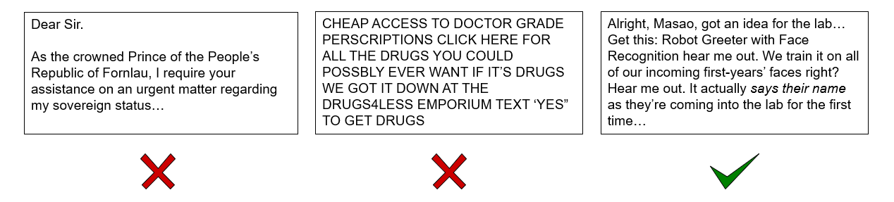
If you were reading an email for the first time, what would be some features that might tip you off as to whether or not the note is Spam v. Ham?
The email address: whether or not the address is someone we know, has a bunch of random numbers in it, is from aol (lol sorry, had to), etc.
The message title: does this subject look legit? Is it something I initiated or that someone sent to me first? etc.
The message text: typos, grammatical errors, CAPS LOCK, plus the words themselves.
All of these are valuable features that could be combined to form a comprehensive machine learning model to predict if any message is Spam or Ham.
We'll focus today on one of the most predictive: the email text itself.
Let's think now for a moment about the actual model we can use to take in words as features from some email and spit out a classification of Spam or Ham.
Naive Bayes Classification
Intuition: let's try to model the probabilistic relationship between the features (the email's words) and the class (Spam v. Ham) using a modified Bayesian Network.
We'll start as we typically do by building some intuition and then look at the specific mechanics of our first approach.
Let's start with an underhand-pitch:
To be effective at predicting some class, what independence relationship should hold between our classifier's features and class variables?
They should be dependent! In other words, knowing about the state of our features should give us information about the state of the class: $$X_i \not \indep Y~\forall~X_i \in X$$
Given this observation, we can start to apply our knowledge about Bayesian Network syntax to consider how to model this scenario.
We know we want our features to be related to our class, but there are really two approaches we could take for modeling the features for classification:
Try to model the conditional independence relationships between the features (the words)
Ignore the conditional independence relationships between features, focusing only on their relationship with the class
What are some problems or challenges with approach #1 when it comes to the task of email classification?
Too many meaningless dependencies! Words often appear with each other, even given the class of Spam v. Ham; most of these dependences will be meaningless to the task at hand, so worrying about the relationships *between* the words rather than between the words and the class seems extraneous.
As such, for classification tasks, we'll investigate option 2: to ignore the possible dependence relationships between features, and see how our model performs.
Given that we want our class variable to be dependent on our features, what possible network configurations could yield this relationship?
There are two choices: (1) features parents of class \(X_i \rightarrow Y\) or (2) class parent of features \(Y \rightarrow X_i\)
Let's consider each of these choices separately.
Features Parents of Class
This modeling approach would look like the following:
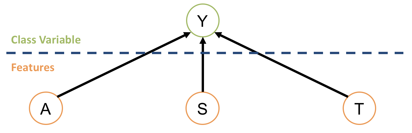
What is the damning problem with this approach?
The size of the CPT for the class variable is the same as the joint distribution! This would grow out of control and be useless for large feature sets.
So, let's consider the alternative:
Class Parent of Features
This modeling approach would look like the following:
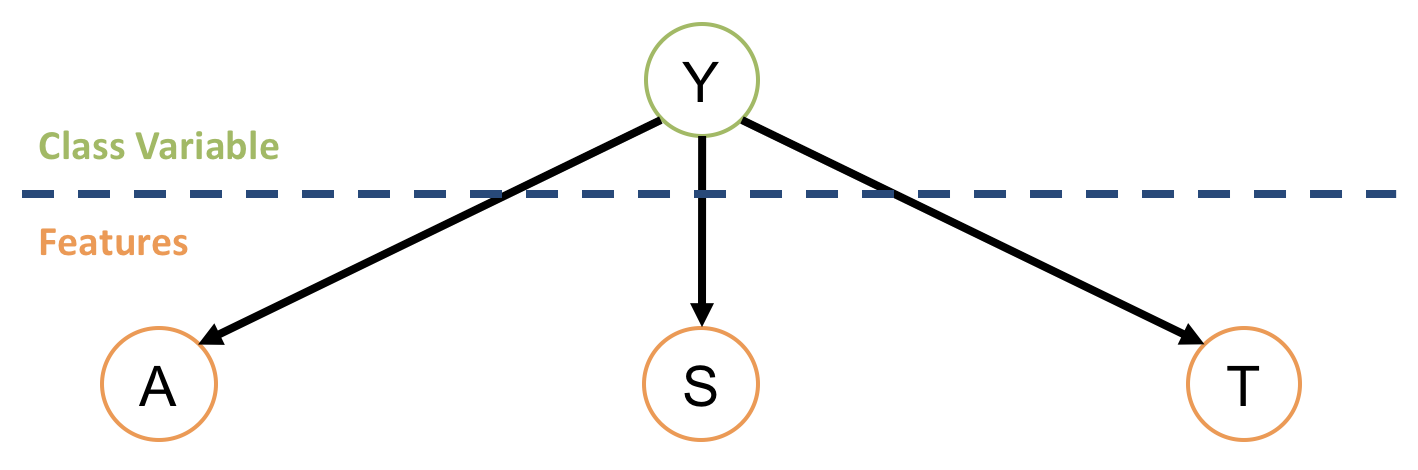
Does this structure suffer the same problem that the last one did? How is it better if not?
No it doesn't! Herein, the largest CPT that needs to be maintained is the feature with the largest number of values, which would (plainly) be less of a memory tax than the alternative.
For this reason, and others, this is the type of model we'll consider for our classifier in what is known as a Naive Bayes model.
Naive Bayes - Structure and Semantics
A Naive Bayes Classifier is a simplified Bayesian Network in which the class variable \(Y\) is a parent to all features \(X_1, X_2, ...\), and can be used to determine which class is most likely given some instantiation of features.
It is considered "naive" compared to the more general Bayesian Network because:
It assumes that all features are independent given the class, i.e., \(X_j \indep X_i|Y~\forall~X_i, X_j \in X\)
It is not meant to answer general inference queries except those that pertain to classification
With this definition, determine: what probabilistic statement would allow us to determine the most likely class \(y \in Y\) given an instantiation of features \(X_1 = x_1, X_2 = x_2, ...\)?
We would attempt to find the class that was most likely given the features, formally: $$argmax_{y \in Y} P(Y = y | X_1 = x_1, X_2 = x_2, ...)$$
Great! So we have a probabilistic expression we can attempt to evaluate... the only problem is that this is not a simple expression to evaluate given our network structure (is certainly not an immediately answerable query).
Is there some tool from probability theory that could take our target maximization quantity and express it in terms of our NBC's parameters?
Yep, Bayes' Theorem! Observe that: $$\begin{eqnarray} P(Y | X_1, X_2, ...) &=& \frac{P(X_1, X_2, ... | Y)P(Y)}{P(X_1, X_2, ...)}~\text{Can be simplified further using NBC structure:} \\ &=& \frac{P(X_1 | Y) P(X_2 | Y) ... P(Y)}{P(X_1, X_2, ...)}~\text{Because features independent given class} \\ \end{eqnarray}$$
Getting closer! Now, consider that a NBC will attempt to find the class that maximizes this quantity, and will conclude that it's the most likely.
As such, consider that we have two classes \(Y = 0, Y = 1\) and are attempting to determine which is more likely for a given instantiation of features. We would be comparing: $$\frac{P(X_1=x_1 | Y=0) P(X_2 = x_2 | Y=0) ... P(Y=0)}{P(X_1=x_1, X_2=x_2, ...)} \stackrel{?}{>} \frac{P(X_1=x_1 | Y=1) P(X_2=x_2 | Y=1) ... P(Y=1)}{P(X_1=x_1, X_2=x_2, ...)}$$
If the LHS is greater than the RHS, we would consider the most likely class to be \(Y = 0\), and vice versa to conclude \(Y = 1\).
However, notice that we can simplify the compared expressions even further; what parts of the above expressions can be ignored during classification?
The denominators \(P(X_1=x_1, X_2=x_2, ...)\) since these will be "constant" in computing the likelihood of all compared classes.
As such, we now have the complete rule for a Naive Bayes Classifier:
A Naive Bayes Classifer will classify (for class variable \(Y\)) some data point corresponding to an instantiation of features \(X_1 = x_1, X_2 = x_2, ...\) by selecting the class that maximizes: $$argmax_{y \in Y} P(X_1 = x_1 | Y = y) P(X_2 = x_2 | Y = y) ... P(Y = y) = argmax_{y \in Y} P(y) \prod_{x_i} P(x_i | y)$$
Note that each of the expressions in the maximization quantity above can be answered directly from a NBC's parameters.
What's a practical concern with the above rule when the number of features is large? What can we do to solve this problem?
Damn computers: floating point issues! Thankfully, we can use basic maths to save the day (story of this class amirite?) Note: $$log(A*B) = log(A) + log(B)$$
As such, NBCs often choose the class that maximizes the log-likelihood such that: $$argmax_{y \in Y} P(y) \prod_{x_i} P(x_i | y) = argmax_{y \in Y}~log(P(y)) + \sum_{x_i} log(P(x_i | y))$$
Bags of Words
What we *haven't* yet discussed is precisely how we model the features in the Spam v. Ham setting.
In general, will the order that words appear in a sentence be important for some *classification* task?
This answer's a bit tricky: in general, it's arguable that "yes" word ordering is important (e.g., in sentiment analysis wherein the order can matter [especially with negations like "not" preceeding some otherwise "good" word]), but in our case, since we're just trying to examine the association between the words and some class, we might be able to get away with the simpler problem of ignoring order.
Intuitively, we can (in pursuit of labeling as spam or not) deduce the likely spam content of the following two sentences, even when, in the second, the order of the words are not grammatically correct:
DRUGS FOR SALE HERE BIG DISCOUNTS
DISCOUNTS FOR HERE DRUGS SALE BIG
As such, for NBCs, we'll adopt a word-order-independent model known as a "bag of words."
In bag-of-words models, each word position \(W_i\) is identically distributed such that, for class \(Y\): $$P(W_i | Y) = P(W_j | Y)~\forall~i, j$$
Let's try a simple example to concrete the ideas above...
Practice
Consider the following NBC that has been trained on a dataset from our motivating advertising engine example, producing the CPTs below:
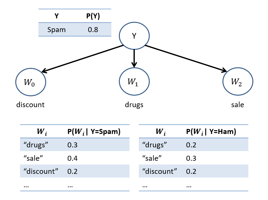
What would we classify a message with the text "discount drugs sale"? Spam \(Y=0\) or ham \(Y=1\)?
Comparing our two classes: $$\begin{eqnarray} P(Y = 0) P(W_0 = discount | Y = 0) P(W_1 = drugs | Y = 0) P(W_2 = sale | Y = 0) &\stackrel{?}{>}& \\ P(Y = 1) P(W_0 = discount | Y = 1) P(W_1 = drugs | Y = 1) P(W_2 = sale | Y = 1) \\ 0.8 * 0.2 * 0.3 * 0.4 &\stackrel{?}{>}& 0.2 * 0.2 * 0.2 * 0.3 \\ 0.0192 &>& 0.0024 \end{eqnarray}$$ Therefore, we conclude that \(Y = 0\) is the more likely class (we assert that this message is spam).
Simple as that! (we could've done the log-likelihood above but just keeping it simple for now)
Other Applications
Naive Bayes Classifiers, despite their simplicity, are used in a variety of other applications as well.
Learning NBCs
Last time, we looked at how to USE NBCs, but not how to construct one from some set of Data.
We should, before that endeavor, take a step back and ask just what we have to learn:
Given our assumptions implicit in defining an NBC, what do we have to learn from data?
The CPT rows / parameters!
Note: by our "naivety" assumption with NBCs, we do *not* need to learn the network structure like we might in a general Bayesian Network since we're assuming that all features are related to the class variable, but are each piecewise independent given the class.
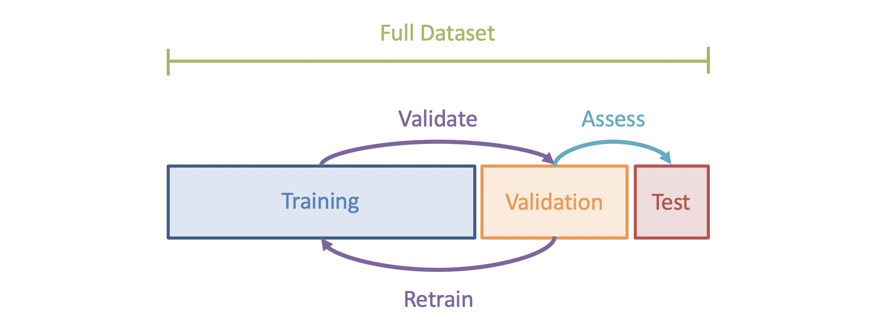
As such, let's consider that we're just at the Training phase in our 3-tiered Experimentation Cycle:
Parameter Estimation
Parameter Estimation is the process of learning some model's parameters (i.e., the variables that will cause it to respond differently to different inputs), usually labeled as \(\theta\), from some training data.
NBC Parameter Estimation is to learn all \(P(Y), P(X|Y)~\forall~x, y\).
How, perhaps as a first, intuitive effort, should we estimate these from data?
Simply count the number of times each co-occur in the training set and then set the parameters to be that ratio!
This technique, although a sort of primitive in parameter estimation, makes a lot of sense: use the training data to make empirical estimates of the data for each event, and is known as the maximum likelihood estimate defined as:
The Maximum Likelihood (ML) Estimate of some event \(x\) is simply the ratio of counts of \(x\), indicated as \(c(x)\) divided by the total number of samples \(N\) (where \(N\) might be restricted by some conditional), viz: $$P_{ML}(x) = \frac{c(x)}{N}$$
We've probably just assumed that we were using ML techniques to populate Bayesian Network / Naive Bayes CPT parameters this whole time -- we were!
It really is that simple to implement too.
How would we apply the ML parameter estimation technique to an NBC on our Spam v. Ham problem?
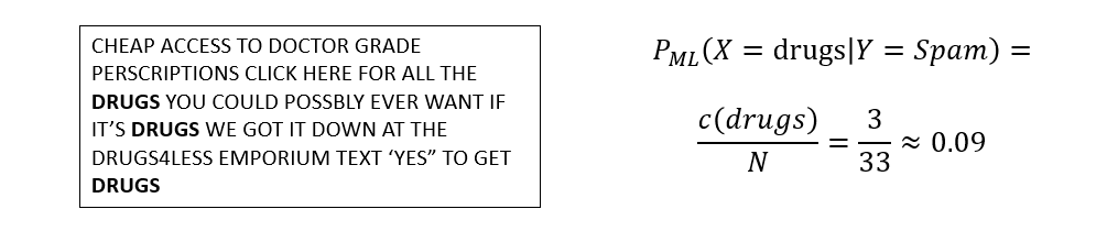
For each email labeled Spam, count the number of times each word appears, divide by the total number, and store in the relevant row in each feature's CPT -- repeat for the other label.
Consider the following example estimating the feature row for the "drugs" word given the Spam label (here, just using a single email with \(N = 33\) words total).
[Reflect] Are there some inherent risks / innacuracies possible by using the Maximum Likelihood technique like this?
Yes, quite a few very important hurdles to overcome:
If we *never* see "drugs" in a *Ham* email, that doesn't mean we should automatically assume that the email is *Spam* (since it might be the case that \(P_{ML}(drugs|ham) = 0\) from our training set).
For example, if the word "drugs" is highly indicative of spam: $$0.5 = P(Y=\text{spam}) * P(X=\text{drugs}|Y=\text{spam}) \gt P(Y=\text{ham}) * P(X=\text{drugs}|Y=\text{ham}) = 0.1$$ ...then including some word like "food" that we've never seen in the training set can unintentionally 0 out both sides: \begin{eqnarray}0 &=& P(Y=\text{spam}) * P(X=\text{drugs}|Y=\text{spam}) * P(X=\text{food}|Y=\text{spam}) \\ &=& P(Y=\text{ham}) * P(X=\text{drugs}|Y=\text{ham}) * P(X=\text{food}|Y=\text{ham}) \end{eqnarray}
In practice, many words will be found in the test set and beyond that were *never* seen in the training set; these shouldn't have 0 probability as well.
Overfitting
The danger of overfitting in machine learning is in creating a model that too closely represents the training set, and is not likely to generalize to samples it hasn't seen before.
Overfitting is like...
...studying for an exam and then being disappointed that the material didn't come exactly from the notes.
...taking entire emails as the only feature in the Spam v. Ham problem (would do really well on the training set but nowhere else).
...being asked to fit a line to some scatterplot and coming up with:
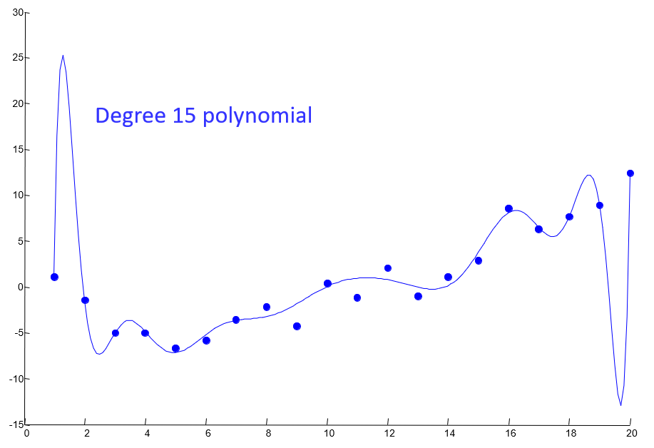
Image credit to Berkeley AI Materials, with permission.
Models that are overfit to the training set will appear to do better than they might "in the real world." Thus, one of the greatest struggles in machine learning is producing a model that both approximates the training set and is likely to succeed in classification outside of it as well.
Insight: avoiding overfitting means sacrificing some accuracy in the training phase with the expectation of greater accuracy in the test phase!
For a NBC using a bag of words parameter estimation, how might we avoid overfitting to the training set?
Smooth parameter estimates to avoid extremes of 0 (impossible for a word to be found with a label) and 1 (a word certainly indicates a label), even if those extremes are found during training.
Smoothing
Smoothing (AKA Regularization) describes techniques used to produce more generalizable models in machine learning by artificially inserting some information.
Smoothing techniques are vast and varried, and we'll look at only one such smoothing technique for our running example.
Note, however, that entire fields of statistics and machine learning have been devoted to finding means of taking some training set, and a learning algorithm prone to overfitting, and perform some sort of smoothing to generalize the model.
Here is one such method that is, once again, surprisingly effective:
Laplace's Estimate: pretend to have seen every outcome once more than was actually witnessed! Thus, for event \(x\), counts of that event \(c(x)\), total samples \(N\), and number of possible values for the variable \(|X|\), we have: $$P_{LAP}(x) = \frac{c(x) + 1}{\sum_x [c(x) + 1]} = \frac{c(x) + 1}{N + |X|}$$
Suppose we are estimating the likelihood of marble color for some \(X \in \{red, blue\}\) in some distribution and witness 2 Red and 1 Blue. Compute our estimate for \(P_{ML}(X = red)\) vs. \(P_{LAP}(X = red)\).
\begin{eqnarray} P_{ML}(X = red) &=& \frac{c(x)}{N} = \frac{2}{3} \\ P_{LAP}(X = red) &=& \frac{c(x) + 1}{N + |X|} = \frac{2 + 1}{3 + 2} = \frac{3}{5} \end{eqnarray}
Some notes on this:
"Smoothing" is an appropriate name because spikes in a distribution are smoothed over and made more uniform (compare 2/3 in the ML estimate above to the more uniform 3/5 in the LAP estimate).
This works for values we may not have seen in the training set as well, wherein \(c(x) = 0\) but some probability mass can still be associated with the event \(x\).
In the case that we have much larger samples, this + 1 is a drop in the ocean, so we may want to smooth even more...
As such, to extend Laplace's Estimate, we can generalize it into:
Laplace's (Generalized) Estimate: pretend to have seen every outcome \(k\) more times than actually witnessed. $$P_{LAP, k}(x) = \frac{c(x) + k}{N + k*|X|}$$ ...and for conditional distributions: $$P_{LAP, k}(x|y) = \frac{c(x, y) + k}{c(y) + k*|X|}$$
All well and good BUT... a reasonable question arises:
How do we know what's best to use for the value of \(k\)?
Learn it!
Tuning
To think about how to learn the value of \(k\) in Laplace's generalized estimate, we first need to distinguish between two different important parts of the learning process:
Parameters are the model's specifications that decide how the function \(f\) maps features \(X\) to classes \(Y\), which are learned from the training data.
In an NBC, the parameters are the network CPTs: \(P(Y), P(X|Y)\).
Hyperparameters are specifications for how the learning of parameters are conducted, which are tuned from the validation data.
In an NBC with smoothing, hyperparameters might include the value of Laplace's \(k\), which can be tuned through repeated experimentation.
This process becomes an optimization problem that looks like the following:
Learn NBC CPTs using a set value of \(k\).
Test this NBC's performance on the validation set.
Revise the value of \(k\) and try again from step 1 until convergence.
Remember the best value of \(k\) and finally assess on test data.
Of what topic / programming paradigm from Algorithms does the above remind you?
Local Search / Hillclimbing! In fact, we had even labeled these as types of approaches for Optimization, but now we're finding some concrete application in the continuous, rather than discrete (e.g., N-Queens, Map-Coloring, etc.), space.
The curve associated with the choice of \(k\) and the model's classification accuracy might look like the following:
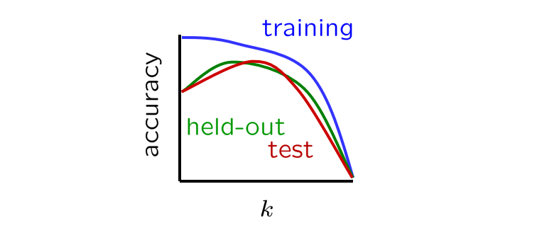
Image credit to Berkeley AI Materials, with permission.
Of note from the above:
When \(k=0\), we overfit to the training data, so with no surprise, accuracy on the training set is maximal when \(k=0 \Rightarrow P_{LAP, k=0}(x) = P_{ML}(x)\)
At the opposite end of the spectrum, for some \(k >> 0\), the model is what we call underfit because we have increased \(k\) so much that the training data is no longer influential on its learned parameters!
As such, the tuning process must find the maximal tradeoff between over and underfitting.
That's a lot of very important ML concepts in a very small nutshell! This is but a tiny introduction to what is an ever widening field, so use this for what it is: a way to get a handle on much of the important vocabulary and techniques that work in a large swath of interesting applications.
Your journey as a data scientist can have a jump start knowing even these basic terms -- and what a journey awaits you!
Next time, we'll switch gears a bit and look at new models that address some of the shortcomings of NBCs.