NBC Shortcomings
Last time, we finished looking at Naive Bayes Classifiers for Bag of Words approaches to spam email classification, but then identified some avenues for improvement:
We might want to include additional features that *aren't* just words (e.g., the sender of the email, if they use your name, the number of capitalized words, etc.), but NBCs are best when features are homogeneous (mingling CPTs on heterogeneous features tricky).
Moreover, some features might be *more* predictive of Spam v. Ham than others, so we should be able to weight their influence accordingly, but NBCs weight all of their features equally (since the CPT values are just probabilities).
In order to address these issues, we'll need some heavier tools, as inspired by some aspects of human neurology.
The Neuron
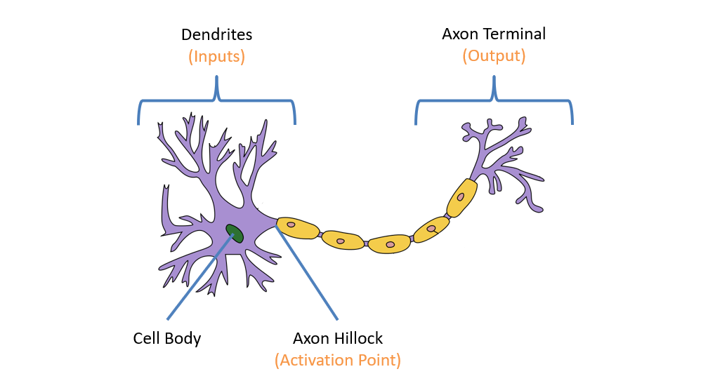
The (rough) components of a neuron are:
Dendrites serve as the neuron's chief inputs, and are also where most other neurons connect across synapses. Neuronal connections vary in strength, with some being more strongly connected than others.
Axon Terminal serves as the neuron's chief output, and can propagate either excitatory or inhibitory signals to any other neurons it is connected to (either increasing or decreasing, respectively, the propensity of a post-synaptic neuron to fire).
Axon Hillock is the part of the neuron that determines if the neuron will "fire" (i.e., send an output signal) to neurons connected to its axon terminals based on its received inputs.
Disclaimer: This is a very brisk over-generalization of the neural structure, and there are many nuances to its behavior that we are still learning about (in fact, new evidence has suggested that it is not so cleanly the basic I/O unit described above).
In brief, neurons are connected to one another, and propagate electrical signals based on some configuration of their inputs.
Take, for example, the famous case of a Jennifer Aniston neuron: a neuron that was measured in some patient's brain to only "fire" when the individual was shown a picture of Jennifer Aniston, but not for other images.
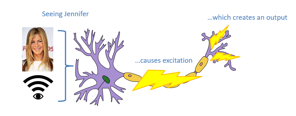
How do we explain the behavior of this Jennifer Aniston neuron? Is it more likely that it is the one neuron in the brain (amongst billions) that happens to be mapped to Jennifer Aniston, or is there a better explanation?
This particular neuron is more of a single gear in a very complex machine -- it is part of the pathway that would be able to discern images of Jennifer Aniston based on its inputs, but it is almost certainly not the only neuron involved in that classification.
Indeed, the true beauty of our brains are not that neurons operate in isolation, but that there is some benefit to their structural organization as a network.
Before we consider this model, however, let's ponder: how can we capture a single element in this complex network? How do we model a single neuron?
Perceptrons
No, that's not the name of the latest protagonist in the endless Transformer's franchise, but instead, has roots to an early approach to machine vision that we'll mimic programmatically today.
Since neurons (or the artificial ones we'll discuss) are functions of their inputs, we need to first think about how to feed input into them and then consider how that input is transformed and then used for classification.
Feature Extraction
Feature Vectors are values corresponding to some selected features that are distilled by a Feature Extractor \(f\) from the raw input \(x\). We'll use the notation \(f_i(x)\) to denote the feature at index \(i\) in the vector returned by the extractor \(f\) that takes a single data point \(x\).
Consider our Spam v. Ham example with a single email input \(x\) that a feature extractor has distilled into whatever quantifiable features \(f(x)\) that we specify.
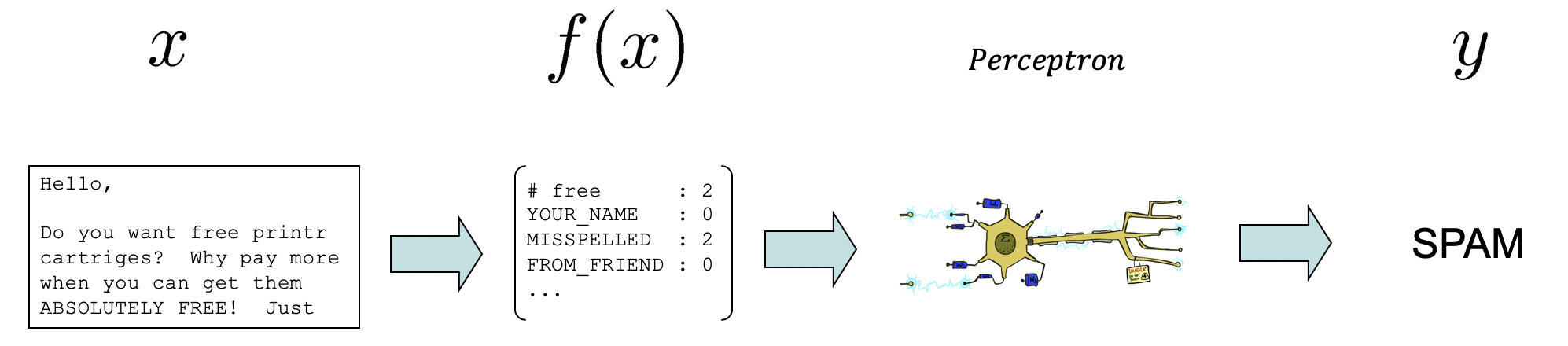
Modified from Berkeley's AI materials, with permission.
Notably from the above, we haven't described *how* the feature extractor gets its vector of features from the raw data, but in the case of text it can be as simple as counting some words that strongly correlate with a class, or binary (0, 1) values for boolean features (e.g., isKnownEmail).
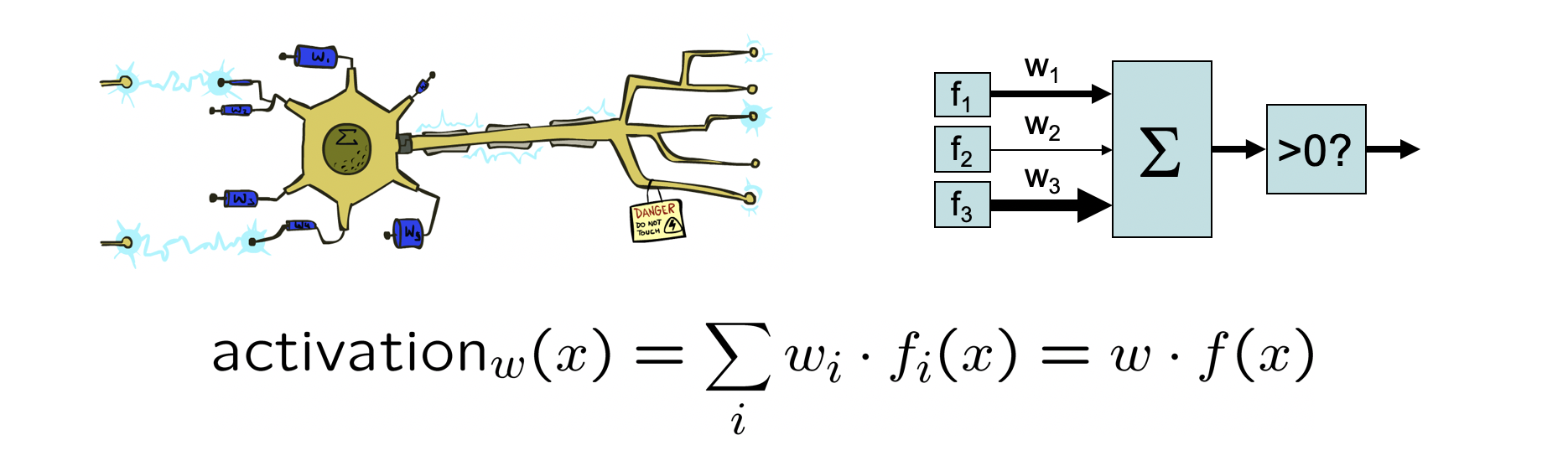
Perceptron Activation
In neuroscience, the process by which "neurons that fire together, wire together" is known as Hebian Learning, and suggests that different neurons have stronger connections the more often they activate at the same time.
This provided the notion that some inputs should be weighted more strongly than others with perceptrons in a classification task!
Similar to how a nerve will "fire," sending some action potential down the cell body to its axon terminals (and thus, produce an "output") we can consider how a perceptron produces an output from a *weighted* sum over its input features.
A perceptron's parameters are defined by the following:
Weight Vector \(w\): each input feature \(f_i(x)\) is weighted by some scalar \(w_i\) based on how much they contribute to the overall classification.
Less influential features will have weights smaller in magnitude.
Weights are signed (can be negative or positive) depending on whether they indicate (positive) or contraindicate (negative) a class.
Activation Function \(a = \text{activation}_w(f(x))\): takes the weight vector \(w\) and input feature vector \(f(x)\) and produces some activation \(a\). In a linear perceptron, \(a = \sum_i w_i * f_i(x)\) which is the dot product \(w \cdot f(x)\).
Decision Rule \(\hat{y} = \text{decision}(a)\): takes the activation \(a\) for a given weighted input, and decides what class label \(\hat{y}\) that should be assigned to the particular input.
Pictorially:
Modified from Berkeley's AI materials, with permission.
Some notes on the above:
When the activation is simply a linear sum of the weighted inputs (which works well for a large swath of problems), we call this a linear classifier.
In the case of a binary class (i.e., \(|Y| = 2\), like for us with Spam v. Not Spam), we have a binary perceptron, and for \(|Y| \gt 2\), we have a multi-class perceptron.
How we formalize the decision rule depends on whether or not we have a binary or multi-class perceptron... so let's think about both to get some intuition!
Binary Decision Rule
Another way of thinking about a decision rule \(\hat{y} = \text{decision}(a)\) is that it is a mapping from activation to class label.
To consider how we might craft a decision rule for a binary classifier, we need to get some intuition surrounding a bit of linear algebra.
Intuition 1: Both the weights \(w = \langle w_1, w_2, ... w_n \rangle\) and extracted features \(f(x) = \langle f_1, f_2, ... f_n \rangle\) are n-dimensional vectors.
Intuition 2: The dot-product between two vectors \(V_1 \cdot V_2 = \sum_i V_1[i] * V_2[i]\) is a single scalar value that is positive when they point in the same direction, and lower when they do not.
\begin{eqnarray} \langle 0, 1 \rangle \cdot \langle 1, 1 \rangle &=& 1 \\ \langle 0, 1 \rangle \cdot \langle 1, -1 \rangle &=& -1 \end{eqnarray}
Intuition 3: Taking the dot product between \(w \cdot f(x)\) will provide a measure of whether or not they're "in the same direction".
Intuition 4: In binary classification, we can consider the weights to be indicative of ONE class \(Y = 0 = \text{spam}\) such that if \(w \cdot f(x) \gt 0\), we would label \(x\) to be equal to \(\hat{y} = 0\), and if it were negative, \(\hat{y} = 1\).
The Binary Perceptron Decision Rule is thus:
$$\hat{y} = (\text{activation}_w(f(x))) \gt 0~?~0 : 1$$
(where the syntax above is the ternary operator: (condition)~?~value_if_true : value_if_false)
Consider the following spam-v-ham visualization for weights indicative of the spam class; inputs (like \(x_1\)) with a positive dot-product will be labeled as spam, and those (like \(x_2\)) with a negative dot-product as ham.
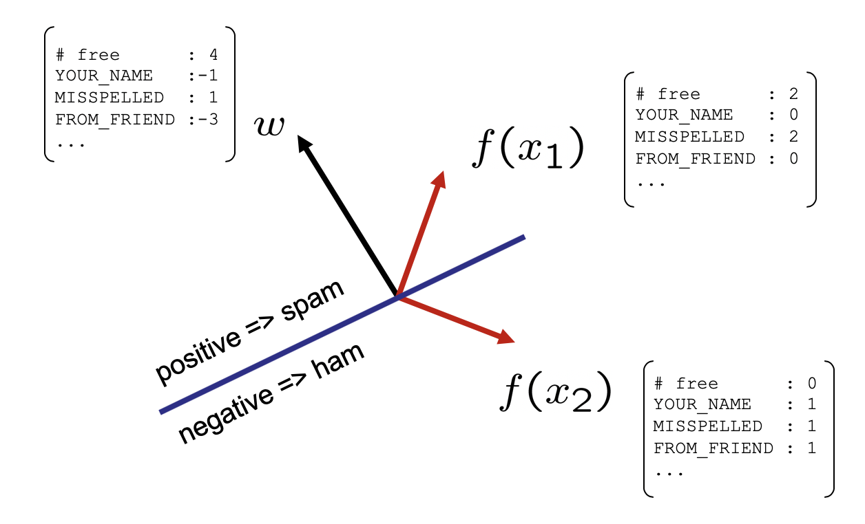
Modified from Berkeley's AI materials, with permission.
Notice the line that separates where we would assign one class versus the other which is known as the decision boundary.
To visualize the behavior of the decision boundary, there's a neat little web app that looks like it was made in the same era that CRT monitors were a hot commodity. Still, you can play around with the behavior of the dot-product between two vectors \(A,B\), pretending that \(A = w\) and \(B = f(x)\):
Example
For the example above, we have \(w = \langle -4, -1, 1, -3 \rangle\) and some extracted features \( f(x_2) = \langle 0, 1, 1, 1 \rangle \), what class should we assign if our decision rule has \(Y = \{\text{spam},\text{ham}\} = \{0,1\}\)?
Step 1: Compute activation \(a = \text{activation}_w(f(x)) = \sum_i f_i(x) * w_i\)
$$f_0(x)*w_0 + f_1(x)*w_1 + ... = -4 * 0 + -1 * 1 + 1 * 1 + (-3) * 1 = -3$$
Step 2: Compare activation output to decision rule:
$$a = -3 \lt 0 \Rightarrow \hat{y} = 1 = Ham$$
Multi-class Perceptrons
Note that the above trick works because we equate one class \(Y=0\) with *positive* activations and the other with *negative* activations. Plainly this trick won't scale in general for \(|Y| > 2\).
That said, we can easily generalize our intuition of the dot-product as being a metric of similarity to some class weights!
For Multi-class Perceptrons (i.e., for ternary class variables and above) generalize the binary case such that:
Each class \(y\) has its own weight vector \(w_y\) that must be record-kept separately.
Each activation for a given sample \(f(x)\) is scored on *all* class weight vectors such that we have \(\text{activation}_{w_y}(f(x))\)
The decision rule / label assigned is corresponds to the class' weight vector most like the sample's features such that: $$\hat{y} = argmax_y~\text{activation}_{w_y}(f(x)) = argmax_y~f(x) \cdot w_y$$
Intuitively, we can think about the decision rules for each type of perceptron as:
Binary: Is my input \(f(x)\) like my weights \(w\) corresponding to class \(Y=0\) or not?
Multi-class: Which of my weights / classes \(w_y\) is my input \(f(x)\) *most* like?
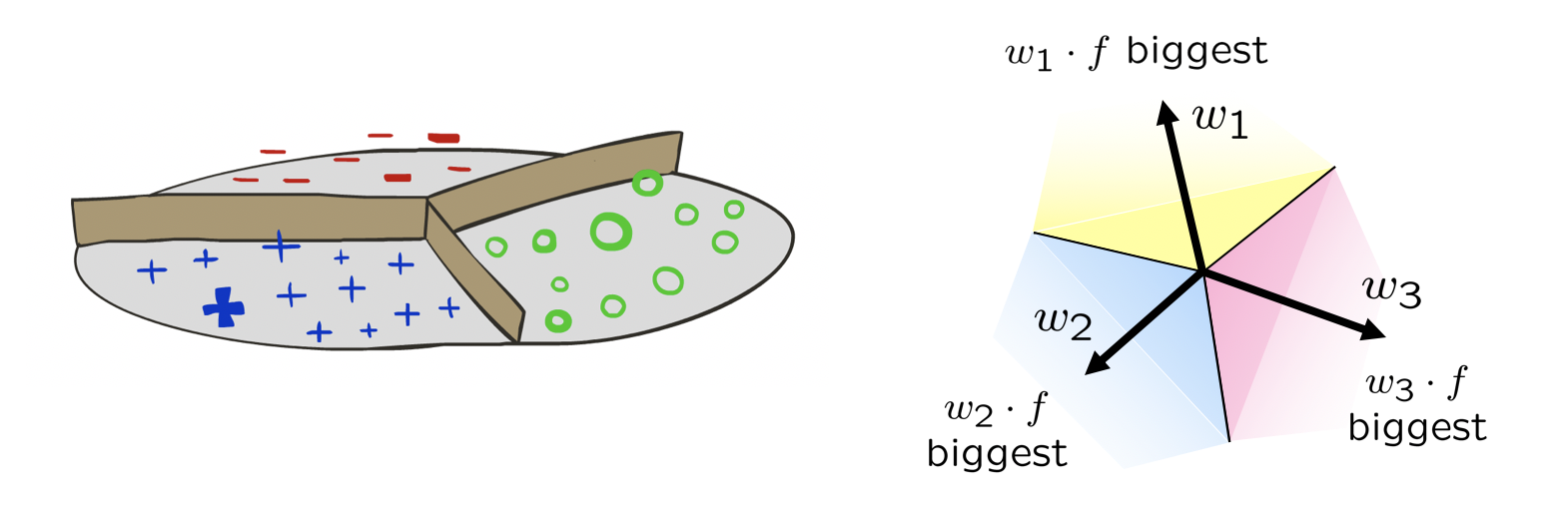
Modified from Berkeley's AI materials, with permission.
Consider the following example scenario with:
3 features, and 3 classes \(\{Y \in \{1, 2, 3\}\}\)
Class weights: \(w_0 = \langle 0, 1, 2 \rangle, w_1 = \langle -1, -2, 0 \rangle, w_2 = \langle 2, 0, 2 \rangle \)
New sample: \(f(x) = \langle 1, 3, 2 \rangle \)
Which class would the perceptron assign to the input \(x\) above?
\begin{eqnarray} \text{activation}_{w_1}(f(x)) &=& 1 * 0 + 3 * 1 + 2 * 2 = 7 \\ \text{activation}_{w_2}(f(x)) &=& 1 * -1 + 3 * -2 + 2 * 0 = -7 \\ \text{activation}_{w_3}(f(x)) &=& 1 * 2 + 3 * 0 + 2 * 2 = 6\\ \therefore \hat{y} = 1 \end{eqnarray}
Learning Perceptrons
What we haven't yet seen is how these weights, and their attachments to the various classes, can be learned, so let's think about that now!
With Perceptrons, much like life, we learn from our mistakes! The gist of learning here is that we (1) attempt to classify each example in the training set, and (2) when wrong, adjust the weights *proportionately to each feature* to make us less-wrong.
Suppose we have 3 classes and weight vectors \(w_1, w_2, w_3\) and misclassify an input \(f(x)\) as \(\hat{y} = 2\) when it should've been \(\hat{y} = 1\). What can we say about the activations \(a_1, a_2\)?
\(a_1\) must've been too low and \(a_2\) must've been too high! So, nudge them in those directions!
By assumption, we start with our known features and classes, and now, have a training set to train the weights... this may be the only weight training that is conducted in computer science (/s).
Linear Perceptron Weight Training
The Basic Linear Perceptron Update algorithm is stated as follows:
  # Initialize all class' weight vectors to all 0s
  w_y = <0, 0, ..., 0>

  # Go through each example in training set
  for each x in training_set:
      # Make prediction with current weights
      y_hat = argmax_y w_y • f(x)

      # Let's call y* the "right" answer from training
      # If our prediction y_hat is right, yay! Do nothing... else:
      if y_hat != y*:
          # Reduce weights of false positive
          w_{y_hat} = w_{y_hat} - f(x)
          # Increase weights of correct answer
          w_y* = w_y* + f(x)
Consider the following example scenario wherein we are midway through some training with:
3 features, and 3 classes
Current class weights: \(w_1 = \langle 1, 0, 2 \rangle, w_2 = \langle -1, 2, 0 \rangle, w_3 = \langle 0, -2, 2 \rangle \)
New sample: \(f(x) = \langle 1, 2, 3 \rangle \), \(y* = 2\)
Compute the update that would occur to weights here.
Step 1: Compute the activation for each class:
\begin{eqnarray} \text{activation}_{w_1}(f(x)) &=& 1 * 1 + 0 * 2 + 2 * 3 = 7 \\ \text{activation}_{w_2}(f(x)) &=& -1 * 1 + 2 * 2 + 0 * 3 = 3 \\ \text{activation}_{w_3}(f(x)) &=& 0 * 1 + (-2) * 2 + 2 * 3 = 2 \end{eqnarray}
Step 2: Select class by decision rule.
$$\hat{y} = argmax_y~\text{activation}_{w_y}(f(x)) = argmax_y~w_y \cdot f(x) = 1$$
Step 3: Update weights if wrong, or keep them if right!
Here, our perceptron said that this sample was \(\hat{y} = 1\) but our correct answer was \(y* = 2\). So we were WRONG and must update (oh the sweet pain of regret):
Penalize the weight of the one that was too high: $$w_{y_{hat}} = w_{y_{hat}} - f(x) = w_1 - f(x) = \langle 1, 0, 2 \rangle - \langle 1, 2, 3 \rangle = \langle 0, -2, -1 \rangle$$
Accentuate the weight of the one that was too low: $$w_{y*} = w_{y*} + f(x) = w_2 + f(x) = \langle -1, 2, 0 \rangle + \langle 1, 2, 3 \rangle = \langle 0, 4, 3 \rangle$$
Some things to note from that example:
That update was pretty extreme! Subtler score adjustments will be a mechanic we discuss in our next toolset.
Try recomputing the example with the new weights -- what do you notice?
The reason we repeat this procedure over the entire training set is to be right on average... even though sometimes we won't be. What might look like an extreme update above might be "mellowed out" as the full training set is sampled
Perceptron Properties
Let's think about some properties of what we've been doing...
Recall from our visualization above that the weight vector's dot product with the features forms one or more decision-boundaries that are linear / planar in nature.
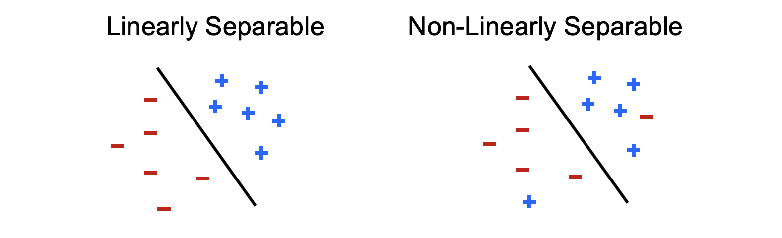
Separability: is a property of the training set if there exists some parameters (i.e., choices of weights) that will perfectly classify each sample within it, meaning that decision boundaries partition the labeled data.
If a training set is separable, the perceptron update rule converges to one such choice for optimal weights.
Above, the black line indicates the decision-boundary formed by a weight vector that would be perpendicular to it and point toward the + direction datapoints.
Modified from Berkeley's AI materials, with permission.
That's a nice property! ...and believe it or not, for many problems, happens more than you might expect, especially because many feature vectors are large, and so there's a lot of space in those dimensions to find a separating set of parameters.
But... there are some problems with perceprons...
Perceptron Problems
As aliterative and whimsical as that sounds, there are a few Perceptron Pitfalls (dammit, did it again) of which we should be aware.
Several issues with perceptrons:
Overtraining: iterating over the training set and updating weights too much will introduce overfitting. Even though accuracy on the training set grows, we start to lose generalizability in the held-out and test sets.
Weight-thrashing: if a training set isn't linearly separable, weights may thrash back and forth without ever finding a good middle-ground that maximizes accuracy.
Mediocre Generalization: if the dataset *is* linearly separable, some decision boundaries will better generalize than others, and the perceptron isn't guaranteed to find the best.
Depicted:
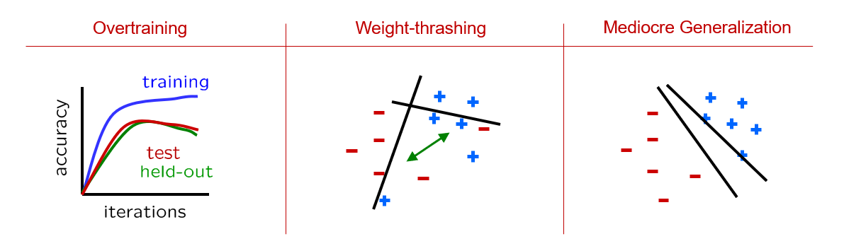
Modified from Berkeley's AI materials, with permission.
It turns out that solving our first problem isn't too bad, but the other two require some finesse...
How might we solve the issue of overtraining?
Just stop training / updating weights as soon as we recognize that accuracy is falling on the held-out set!
Next lecture, let's think about how to tackle thrashing and mediocre generalization!