Fixing Perceptrons
Let's revisit the issue the haunted us with linear Perceptrons: the notion of non-separability (depicted below in the binary class case):
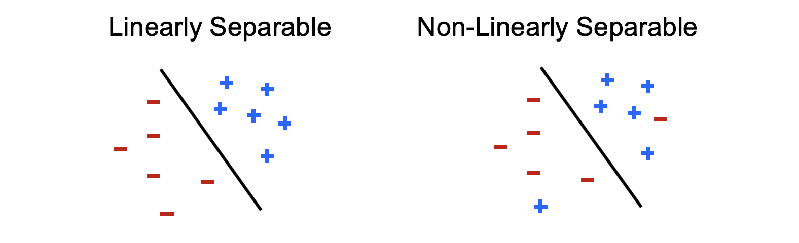
Above, the black line indicates the decision-boundary formed by a weight vector that would be perpendicular to it and point toward the + direction datapoints.
Modified from Berkeley's AI materials, with permission.
Reasonably, you might observe...
Going out of our way to accommodate the few outliers compromises our generalizability and makes us likely to overfit!
There might be other scenarios where we *want* to overfit given a large enough training set, but with the complexities of the problems we're currently looking at (which hand-made feature extractors), we'll often get in more trouble going out of our way to accommodate outliers.
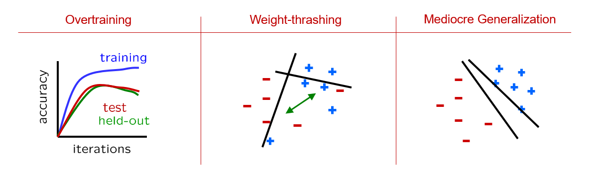
Still, we need some way of avoiding the last two issues we discovered with Perceptrons, viz., thrashing (for non-linearly separable training sets) and mediocre generalization, depicted again below:
Modified from Berkeley's AI materials, with permission.
Intuition: Notice how the two issues we didn't solve last time (viz., thrashing and mediocre generalization) are a consequence of over-adjusting the weights whenever the perceptron misclassified a sample.
How can we make a tweak to the perceptron's decision boundaries to get around this "either wrong or right class" paradigm?
Perhaps we can find a way to think of the likelihood of a data point belonging to one class or another to once again give us some shades of gray where previously we'd seen absolutes!
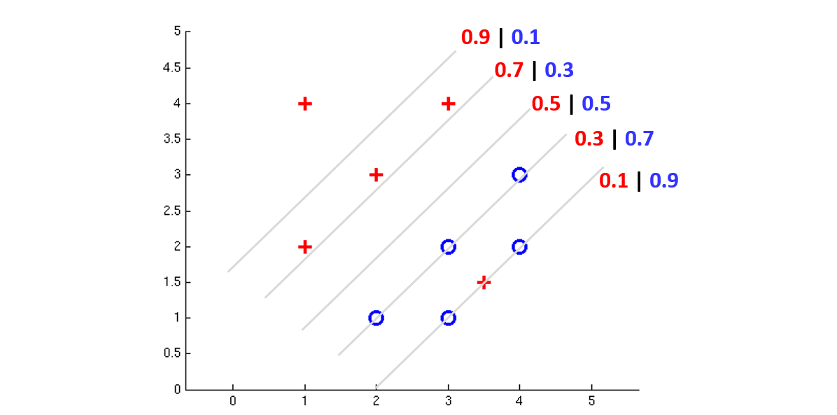
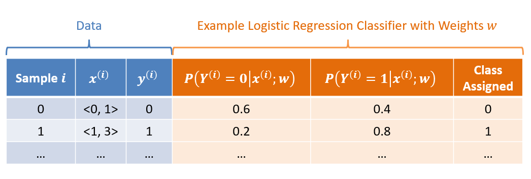
Making this tweak for the following example binary classifier might mean each decision boundary now encodes a *likelihood* of samples on each side belonging to one class over the other:
Modified from Berkeley's AI materials, with permission.
Noting some components from the above:
Here we have *probabilistic* decision boundaries that each have some confidences that (in red) the positive class lives on this line and (in blue) the negative class lives on this line.
So, the trick in this situation is answering the question: "How do I position my decision boundary to best reflect my training data, as now informed by these likelihoods?"
To motivate that endeavor, which of the decision boundaries above seems to best partition the data?
The one in the middle with the 50/50 split! This suggests that we've found the decision boundary that most evenly divides our data.
So... how do we go about finding this boundary and the weight vector that characterizes it?
Logistic Regression
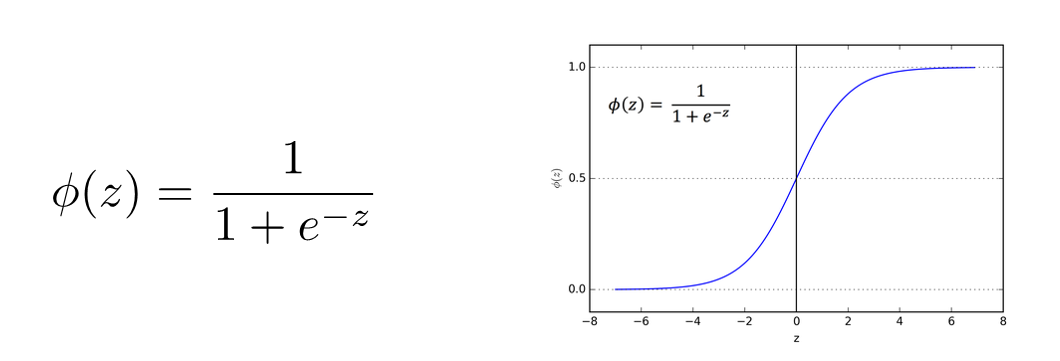
Logistic Regression is a machine learning tool to assign some likelihood that a sample \(X\) belongs to a given class \(y\), which operates like a perceptron except that its activation \(\phi(z) = \sigma(z) = \text{activation}_w(f(x))\) is converted to a likelihood by the sigmoid function (the inverse of the logit function, its namesake).
The sigmoid function, \(\phi(z) = \sigma(z)\), takes any value \(z \in (-\infty, \infty)\) and converts it to a likelihood between \((0, 1)\) where the more negative \(z\) is, the more unlikely the probability, and vice versa for highly positive \(z\).
Depicted, this looks like the following:
Modified from Berkeley's AI materials, with permission.
Insight 1: consider that \(z\) is a linear perceptron's activation (below, as indicated for a binary class, but can be extended to multiple classes later): $$z = w \cdot f(x)$$ ...This means that the likelihood, for the sample \(i\), of the positive class \(y^{(i)} = +1\) given the input \(x^{(i)}\) and choice of weights \(w\) is: $$P(y^{(i)} = +1 | x^{(i)}; w) = \frac{1}{1 + e^{-z}}$$
How does this help us? Well, this lets us compute the likelihood of a given class given the features, even in a continuous space!
Consider if \(z = w \cdot f(x) = 3\). This means that the likelihood, for the sample \(i\), of the positive class \(y^{(i)} = +1\) given the input \(x^{(i)}\) and choice of weights \(w\) is roughly \(0.95\) (i.e., very likely), written: $$P(y^{(i)} = +1 | x^{(i)}; w) = \frac{1}{1 + e^{-z}} = \frac{1}{1 + e^{-3}} \approx 0.95$$
Of course, having a probability that a sample \(X\) belongs to a class \(y\) is only useful if it leads to some classification rule, which is simple in the binary case: just see which class is more likely!
Logistic Regression Binary Decision Rule: since we only have 2 values for \(y\) (think: spam vs. ham), to classify any given input \(x\), we need only see whether the likelihood above is greater than, or less than 0.5 (i.e., which class is more likely given the sample?). In other words, for assigned class \(\hat{y}\): \begin{eqnarray} \hat{y} = \begin{cases} +1, & \text{if $P(y^{(i)} = +1 | x^{(i)}; w) \gt 0.5$} \\ -1, & \text{otherwise} \end{cases} \end{eqnarray}
Multi-class Extension: In order to extend the above definitions into multi-class logistic regression, we can perform the following:
Compute the activations for each class \(y \in Y\): $$z_y = w_y \cdot f(x)$$
Normalize each computed likelihood by what is known as the softmax function, the multi-class generalization of the sigmoid, defined as: $$P(y^{(i)} | x^{(i)}; w) = \frac{e^{z_y}}{\sum_{y'} e^{z_{y'}}}$$
Consider the following softmax outputs for 3 original activations \(z_1, z_2, z_3\):
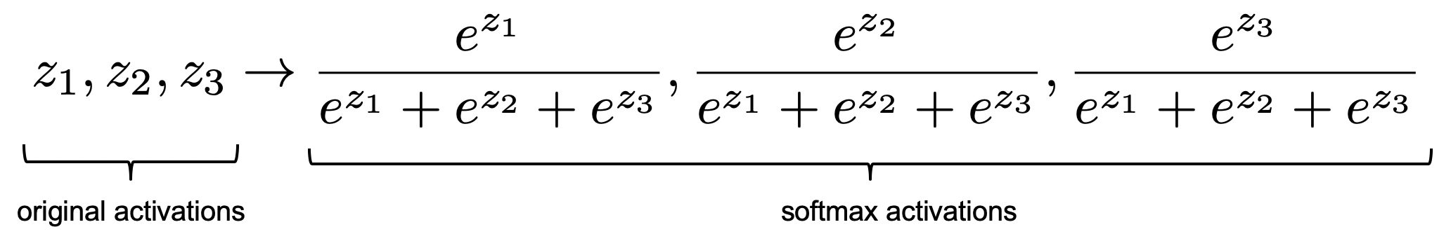
Modified from Berkeley's AI materials, with permission.
Above:
Note that each of the \(\frac{e^{z_y}}{\sum_{y'} e^{z_{y'}}}\) form a vector whose contents sum to 1.
Our decision rule is not much changed from before: instead of just comparing whether or not one class' likelihood is "more likely than not" (above 50 percent), we just look for the greatest and use that to classify.
Logistic Regression Multiclass Decision Rule: for input sample \(x^{(i)}\), assign class \(y\) such that: $$\hat{y}^{(i)} = argmax_y~P(y | x^{(i)}; w)$$
Having a decision rule is good, but we also need some target to aim for that characterizes what set of weights will be the best one in this new context.
Insight 2: Because of this ability to compute likelihoods from activations, we now also have a goal / characterization for what choice of weights is the best for the entire training set!
Suppose we have some training set composed of labeled data (i.e., \((X^{(i)}, y^{(i)})\) pairs); how would we *characterize* the best choice of weights, \(w^*\), given the new probabilistic formalization of a classifier above?
Find the weights that *maximize* the likelihoods of classifying each sample as the *correct* one!
Note: we want the set of weights that successfully classifies as much as possible across *all \(i\) samples*, not just weights that get a few samples right on the nose!
Logistic Regression Maximum Likelihood Weight Estimation: the maximum likelihood choice for weights in logistic regression is characterized as the value for the weight vector \(w\) that maximizes the log-likelihood of the correct class \(y^{(i)}\) across all \(i\) samples in the training set, viz: \begin{eqnarray} w^* &=& \text{\{choose best weights w\}}\text{\{that maximize the log-likelihood of correct class across all i samples\}} \\ &=& argmax_w \sum_i log~P(y^{(i)} | x^{(i)}; w) \\ &=& argmax_w~ll(w) \\ \end{eqnarray}
Remind me: what's the purpose of Log-Likelihoods again?
Avoids numerical underflow from floating-point errors! Without it, we'd be multiplying a bunch of small probability values together. It turns out this will have another benefit later for how we learn logistic regression classifiers.
Consider the softmax function output for input feature vectors in a training set \(f(x^{(i)})\) and then two competing *sets* of weights over 3 classes: \(w, w'\). Then, comparing several datapoints from a training set in which we know the correct \(y^{(i)}\), determine which set of weight vectors we would prefer?
Sample |
\(P(Y^{(i)} | x^{(i)}; w)\) for \(w = \{w_1, w_2, w_3\}\) |
\(P(Y^{(i)} | x^{(i)}; w')\) for \(w' = \{w_1', w_2', w_3'\}\) |
\(y^{(i)}\) (Training Set Label / Correct Answer) |
\(i = 1\) |
\(\langle 0.3, 0.5, 0.2 \rangle\) |
\(\langle 0.5, 0.4, 0.1 \rangle\) |
\(y^{(1)} = 1\) |
\(i = 2\) |
\(\langle 0.2, 0.7, 0.1 \rangle\) |
\(\langle 0.1, 0.5, 0.4 \rangle\) |
\(y^{(2)} = 3\) |
Let's see which set of weights we'd prefer: \(w\) or \(w'\):
Note: it's common during implementation to use the natural log (ln = log_e) to compute the log-likelihood.
\begin{eqnarray} ll(w) &=& \sum_i log~P(y^{(i)} | x^{(i)}; w) \\ &=& log(0.3) + log(0.1) \\ &\approx& -3.50 \\ ll(w') &=& \sum_i log~P(y^{(i)} | x^{(i)}; w') \\ &=& log(0.5) + log(0.4) \\ &\approx& -1.60 \\ &\therefore& \text{Prefer } w' \end{eqnarray}
Some things to note on the above:
We consider the likelihood output for the label class by our softmax regression weights, ignoring the likelihoods of classes that did not correspond to the label.
Even though we prefer the second set of weights \(w'\), it still gets the 2nd sample wrong! Still, it is more in-line with what the training set is telling us to model than the first set of weights, under the assumption that over many such samples, it will learn the happy medium of a decision boundary.
*Neither* of the above sets of weights are *maximal*, which is now the trick for us to find...
All of the above has been to merely *describe* what good weights look like; let's now turn our attention to *how* we might find the value of \(w^*\) that satisfies the maximum likelihood estimation criteria specified above.
Optimization
What we have in finding the weights that maximizes the log-likelihood is what's known as an optimization problem in which we have some continuous values that must be "tweaked" until the best combination is found.
Hillclimbing approaches are common solutions to optimization problems, which follow several basic steps:
Make a random, initial guess for the variables of interest.
Make a change to that state of variables into one of the "neighboring" states that improves your "score" on the problem.
Quit when no neighbors are better than your current state.
Recall the Map Coloring Problem (a Constraint Satisfaction Problem) wherein the goal is to "color" the nodes in a graph such that no two adjacent nodes share the same color.
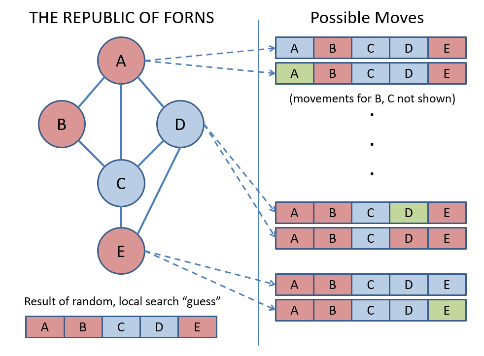
Why do Hillclimbing approaches in the Map Coloring problem not precisely scale to our current endeavor of finding the best weights for logistic regression?
Because they're discrete states whereas we now have continuous weight vectors to learn -- neighborhoods are infinite in size!
The continuous aspect of the current problem actually ends up being a not-totally-hopeless property for one key reason... let's expose why with a simple hillclimbing example in 1 dimension.
1-Dimensional Optimization
Consider that we have some function \(g(w)\) for which we are trying to find the value of \(w\), a single variable, that maximizes \(g(w)\).
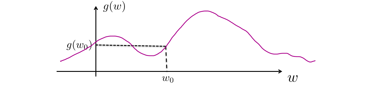
Modified from Berkeley's AI materials, with permission.
If we randomly start with \(w = w_0\), how would we know which direction to move it in order to get closer to a local maximum?
Take the derivative and move in the direction of positive slope! Calculus saves the day again! Namely, compute: $$\frac{\partial g(w_0)}{\partial w}$$
Insight 1: a calculus reminder that derivatives can help us understand "which way is up/downhill" of a function -- that will come in useful later!
Note: Here's where continuous optimization is actually quite nice! We wouldn't be able to compute the derivative of a discrete optimization problem -- it's like having a sherpa guide our search for the best \(w\)!
Suppose we are trying to maximize some function \(g(w_1, w_2)\), now a function of multivariate input.
The same strategy that we used above applies, but now, our updates to the input weights are a little trickier since changes to each one individually might give us a different slope of the multi-dimensional hill to climb.
As such, we'll compute the slopes of each weight change to the function individually, and then combine to find the best (i.e., the steepest-upward) direction to climb.
The tool from calculus that allows us to do this is the partial derivative: $$\frac{\partial g(W)}{\partial w_i}$$ which assesses the rate of change (slope) of some function \(g\) as one of its inputs \(w_i\) changes, treating the other parameters as constants.
If you haven't had Calc 3, believe it or not, partials are pretty painless (and that was alliterative so you know it's true).
Suppose we have MULTIPLE weights and function \(g(w_1, w_2) = 5 w_{1}^2 + 4 * w_2\); compute \(\frac{\partial g}{\partial w_1}\) and \(\frac{\partial g}{\partial w_2}\)
\begin{eqnarray} \frac{\partial g}{\partial w_1} &=& 10 w_1 \\ \frac{\partial g}{\partial w_2} &=& 4 \end{eqnarray}
The combination of these individual partial derivatives is known as the gradient \(\nabla\), a vector that looks like:

Modified from Berkeley's AI materials, with permission.
Insight 2: Now, imagine that the function \(g(w)\) above is our log-likelihood goal \(ll(w)\) -- we'll just try to keep climbing the log-likelihood (multi-dimensional) hill until we find some optimum for the weights!
Some notes:
This approach is called gradient ascent of \(ll(w)\), and for Logistic Regression, will *always* find the global maxima because \(ll(w)\) is known as a convex function.
More common, and applicable outside of just logistic regression, is another algorithm we'll see next...
Insight 3: being more right is the same as being less wrong!
Insight 4: Since we are trying to learn the weights (one for each feature), we can think about starting someplace random and nudging them in directions to be less wrong!
In other words, as opposed to trying to climb uphill of a function that tells us how right we are, consider descending *downhill* of a function that tells us how *wrong* we are.
Here's a visualization of that last insight on a completely unrelated video just showing a 3D figure where we might imagine x and z as features and y as some metric of "how wrong we are."
Logistic Regression - Learning
Although in the above we have given ourselves a target to aim for, we currently lack a couple of things:
An algorithm for learning the weights for logistic regression that fixes the issues with linear perceptron learning.
A way to connect our optimization criteria to the training data in a way that will be computationally feasible.
It turns out there's one idea that helps us do both -- prepare to have your minds blown:
Insight 1: Maximizing how much you're correct is equivalent to *minimizing* how much you're wrong.
What's nice about the remark above is that it relates a bit to how we approached the mistakes we made in our perceptron update rule... but now with probabilities!
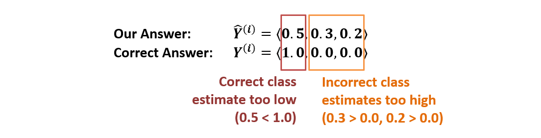
Returning to our ternary email classifier with \(Y \in \{\text{spam = 0, ham = 1, important = 2}\}\) and wherein we have 3 features forming a vector: \(f(x) = \langle f_0(x), f_1(x), f_2(x) \rangle\), and for a sample \(X^{(i)}\), our classifier's activations are \(P(\hat{Y^{(i)}}|x^{(i)}; w) = \langle 0.5, 0.3, 0.2 \rangle\).
If the correct label is \(y^{(i)} = 0\), what, in the best possible scenario, should the \(P(\hat{Y^{(i)}}|x^{(i)}; w)\) outputs / vector look like?
We would like it to be *certain* of the sample being the correct class, and *certain* of the sample *NOT* being the other classes, viz.: $$Y^{(i)} = \langle 1.0, 0.0, 0.0 \rangle$$ (note that the 1.0 appears in the 0th index because the correct answer was \(y^{(i)} = 0\))
A vector like the above wherein all elements are 0.0 except for 1, which has a value of 1.0 is known as a one-hot vector.
Insight 2: Just like a unit test wherein we compare (expected, actual) outputs of some method, we can now correct for the weights
of *each* class based on whether their probability estimates were too low or high!
Here's a depiction of the learning task at-hand if, e.g., class \(y^{(i)} = 0\)) is the correct class for sample \((i)\):
Combining insights 1 and 2 gives us what is called a Loss / Cost Function \(Loss(Y^{(i)}, \hat{Y}^{(i)}) = Loss(\text{expected},\text{actual})\), which provides a metric for how distant our model's output likelihood for each class \(\hat{y}^{(i)} = y^{(i)}\) is from the correct one-hot vector.
The loss function we'll employ for learning our logistic regression model's weights stem from our maximization goal; as a reminder, our maximization goal is the log-likelihood: $$ll(w) = \sum_i log~P(y^{(i)} | x^{(i)}; w)$$
For Logistic Regression (and other models we'll see next time), a common Loss Function is what's known as Cross Entropy (CE) Loss \(Loss_{CE}\) and stems from our log-likelihood weight maximization goal \(ll(w)\): it is defined (for a single sample \(i\)) as the negated log-likelihood of the *correct* class \(y^{(i)}\) from our model's current choice of weights \(w\): \begin{eqnarray} Loss_{CE}(y^{(i)}, \hat{y^{(i)}}) &=& \text{How far from certain our } \hat{y^{(i)}} \text{ was for a single sample i} \\ &=& -log(P(\hat{y}^{(i)} | x^{(i)}; w)) \\ \end{eqnarray}
In our example above, for 3 classes, find the \(Loss_{CE}(y^{(i)} = 0, \hat{y^{(i)}})\) given that \(P(\hat{y^{(i)}} | x^{(i)}; w) = \langle 0.5, 0.3, 0.2 \rangle\) and noting that the correct answer is class \(y^{(i)} = 0\).
\begin{eqnarray} Loss_{CE}(y^{(i)} = 0, \hat{y^{(i)}}) &=& -log(P(\hat{y^{(i)}} = 0 | x^{(i)}; w)) \\ &=& -[log(0.5)]~~~\text{# Usually natural log is used here (i.e., ln = log_e)} \\ &\approx& 0.70 \end{eqnarray}
Some notes on the above:
What does this 0.7 signify? Well, it's a measure of "entropy", which is a bit out of scope to discuss in this class, but is intuitively a measure of distance that our assigned likelihood / confidence in the true class was compared to the ideal case wherein we're 100% confident in it. The greater the distance, the more adjustment we'll need to do.
Note how this loss function behaves if we get the answer right on the dot: if our guess for \(P(\hat{Y^{(i)}} = 0 | x^{(i)}; w) = 1.0\) then we would end up taking \(log(1.0) = 0\), or in other words, our confidence in classifying the sample with the correct class was flawless / had a distance of 0.
Gradients
Here's the roadmap for our weight updates:
The best weights are those that minimize the Loss across all samples in our training set (i.e., are least wrong), which is the same thing as maximizing our log-likelihood across all training samples.
Taking the derivative of a function tells us its slope; taking the *partial* derivative of a multivariate function with respect to one of its variables tells us the slope of just that variable with all others held constant.
If we take the partial derivative of the Cross Entropy Loss *with respect to the weights*, we can learn, with each sample, the direction to *nudge* those weights to be better!
Addressing this final part of the roadmap provides the gradient, i.e., a vector of the derivatives of each weight for the loss function.
The derivative of \(L_{CE}\) with respect to the weights of each class \(w_{k,i}\) (for class \(y = k\)) for a single sample \(i\) is actually quite neat, and is represented as: $$\frac{\partial L_{CE}}{\partial w_{k,i}} = -[1(k = y^{(i)}) - P(\hat{y^{(i)}} = k | x^{(i)}; w)] * x^{(i)}$$ ...where \(1(\hat{y} = y^{(i)})\) is known as the "indicator function", which is 1 when the condition is true (in this case, if \(k\) is the correct class \(y^{(i)}\)), 0 otherwise.
Notes on the above:
The difference \(1 - P(\hat{y}^{(i)} | x^{(i)}; w)\) will be larger the farther our correct class likelihood is from 1, and larger for when our incorrect class labels are farther from 0.
This is the key differentiator from the linear perceptron update rule since we can gradate by how much we nudge each feature's weights!
This difference is also negative, because the slope we're getting back by the derivative takes us uphill, when in fact we want to *minimize* the loss by going the opposite way.
We weight by the inputs \(x^{(i)}\) (these would be the sign and magnitudes of the extracted features) just like in our linear perceptron updates so that each feature's weight gets updated proportionate to how much that feature \(x^{(i)}\) was "active".
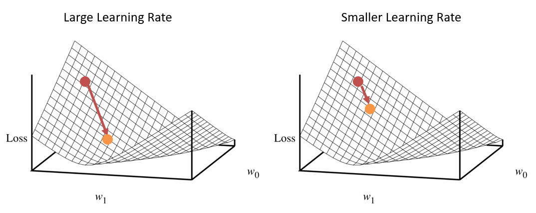
Logistic Regression Weight Update Rule: for a single sample \((X^{(i)}, y^{(i)})\) weights belonging to each class \(w_{y}\) can be nudged in the "more correct" direction for some learning rate hyperparameter \(\eta\) that is typically a small fraction to ensure we do not overshoot the minimum of the loss during hillclimbing: $$w_{k,i} = w_{k,i} - \eta * \frac{\partial L_{CE}}{\partial w_{k, i}}$$
Notes on the above:
Notice that we subtract from the weight's current value because we want to go in the direction *opposite* of the slope so as to go "downhill".
As a result of nudging the weights of the correct class to be greater by some proportionate amount, the likelihoods of the correct class given that input goes up, and the likelihoods of the incorrect classes given that input go down (since the normalizing denominator of the softmax function is larger).
Why the learning rate? Let's consider a depiction wherein, if we're nearing the minimum of the Loss, we don't want to nudge the weights by too much that we're constantly "jumping" over the global min:
Stochastic Gradient Descent [SGD] (Nutshell)
Why can't we just analytically compute the maximum of the Loss function to find the best weights like we do in Calculus?
Because we'd have to do so for *huge* training sets and often large feature vectors, which is computationally infeasible.
Instead, we can apply our hillclimbing approach to some nice effect.
Combining all of the above gives us an algorithm known as Stochastic Gradient Descent whereby we start at some small random / 0 value of weights, and with each sample in the training set, nudge the weights to minimize the Loss (i.e., go down the gradient of the Loss function).
SGD gets its name since we are taking incremental "steps" to minimize the Loss by nudging the weights after seeing samples in random order one at a time.
The general steps of SGD are:
  initialize w_y = <0, 0, 0, ...>

  while validation set accuracy still increasing:
      for each sample (X^(i), y^(i)) in training set (in random order):
          compute P(Y|x^(i); w)
          compute gradient (derivatives) of Loss_CE for each w_{k,i}
          update weight of each class: w_{k,i} = w_{k,i} - learning_rate * gradient
Some notes on the above:
The
learning_rateis that small constant \(\eta\) that ends up being a hyperparameter used to make sure the weight adjustments aren't too large such that they miss the minimum of the Loss.Note that *ALL* weights update with each inner-loop iteration, unlike the linear perceptron update rule.
Unlike the linear perceptron update weight training algorithm, we end up solving pretty much all of our problems from before:
Mediocre Generalization: because weights are changed based on the gradient, and gradually based on the learning rate, we'll "settle" with decision boundaries that are not biased towards certain classes over others.
Weight Thrashing: solved by having a learning rate.
Overtraining: solved by having an outer loop "converge" on the most generalizable weights by periodically checking in with the validation set.
Consider a small example with the following details:
3 classes: \(Y \in \{0, 1, 2\}\)
2 features, 2 weights per class
Current class weights: \(w_0 = \langle -1, 1 \rangle\), \(w_1 = \langle 1, -2 \rangle\), \(w_2 = \langle -2, 2 \rangle\)
A sample \(X^{(i)} = \langle 2, 1 \rangle\) with label \(y^{(i)} = 1\) and learning rate \(\eta = 0.1\) (actually quite large).
Warning: the below is laboriously calculated so you get a feel for what the algorithm's doing -- this would, in practice, be parallelized into linear algebra!
Step 1: Compute \(P(Y|x^{(i)}; w)\) (the output likelihoods for each class given the current inputs \(x^{(i)}\))
\begin{eqnarray} z_0 &=& w_0 \cdot x^{(i)} = -2 + 1 = -1 &\Rightarrow& e^{z_0} &\approx& 0.36 \\ z_1 &=& w_1 \cdot x^{(i)} = 2 - 2 = 0 &\Rightarrow& e^{z_1} &\approx& 1.00 \\ z_2 &=& w_2 \cdot x^{(i)} = -4 + 2 = -2 &\Rightarrow& e^{z_2} &\approx& 0.14 \\ \end{eqnarray} \begin{eqnarray} P(\hat{Y}=k|x^{(i)}; w) &=& \frac{e^{z_{k}}}{\sum_{y'} e^{z_{y'}}} \\ &=& \langle \frac{0.36}{0.36 + 1.00 + 0.14}, \frac{1.00}{0.36 + 1.00 + 0.14}, \frac{0.14}{0.36 + 1.00 + 0.14} \rangle \\ &\approx& \langle 0.24, 0.67, 0.09 \rangle \end{eqnarray}
Step 2: Compute gradient of Loss for each class:
\begin{eqnarray} \frac{\partial L_{CE}}{\partial w_{k,i}} &=& -[1(k = y^{(i)}) - P(\hat{Y^{(i)}} = k | x^{(i)}; w)] * x^{(i)} \\ \frac{\partial L_{CE}}{\partial w_{0,i}} &=& -[1(0 = 1) - P(\hat{Y^{(i)}} = 0 | x^{(i)}; w)] * x^{(i)} \\ &=& -[0 - 0.24] * \langle 2, 1 \rangle \\ &=& \langle 0.48, 0.24 \rangle \\ \frac{\partial L_{CE}}{\partial w_{1,i}} &=& -[1(1 = 1) - P(\hat{Y^{(i)}} = 1 | x^{(i)}; w)] * x^{(i)} \\ &=& -[1 - 0.67] * \langle 2, 1 \rangle \\ &=& \langle -0.66, -0.33 \rangle \\ \frac{\partial L_{CE}}{\partial w_{2,i}} &=& -[1(2 = 1) - P(\hat{Y^{(i)}} = 2 | x^{(i)}; w)] * x^{(i)} \\ &=& -[0 - 0.09] * \langle 2, 1 \rangle \\ &=& \langle 0.18, 0.09 \rangle \\ \end{eqnarray}
Step 3: Update weights of each class:
\begin{eqnarray} w_{k} &=& w_{k} - \eta * \frac{\partial L_{CE}}{\partial w_{k}} \\ w_{0} &=& \langle -1, 1 \rangle - 0.1 \langle 0.48, 0.24 \rangle &=& \langle -1.048, 0.976 \rangle \\ w_{1} &=& \langle 1, -2 \rangle - 0.1 \langle -0.66, -0.33 \rangle &=& \langle 1.066, -1.976 \rangle \\ w_{2} &=& \langle -2, 2 \rangle - 0.1 \langle 0.18, 0.09 \rangle &=& \langle -2.018, 1.991 \rangle \\ \end{eqnarray}
Notes on the above:
In step 2, the gradient actually said that the way "uphill" was to reduce the weights -- but remember that we're trying to *minimize* the Loss, so we negate it / go the other way when we update the weights in step 3.
When we do eventually update the weights, note that they got nudged up, because increasing these values will get us closer to the 100% confidence that class y=1 is the correct one for samples looking like the input X.
If we repeat this a bunch of times for the samples in our training set, eventually we'll hit some optimum, being sensitive not to overtrain and lose accuracy in the validation set!
Note that above the learning-rate is fixed for the pseudocode of SGD, but what would make sense to do with later iterations of the weight updates?
Slowly attenuate the learning-rate, making it smaller for later iterations so we make sure not to miss the minimum of the Loss!
Comparisons to Perceptrons / NBCs
In practice, the only thing we really lose by using Logistic Regression rather than a Linear Perceptron is time!
It turns out that training via SGD can take quite a few iterations, and though it avoids the issues that Perceptron learning suffered, it can take nontrivial time for large feature sets.
Perceptrons: simple, can be customized with different activation functions, and learning is fast when data is separable.
Logistic Regression: more interpretable with likelihoods assigned to each class, takes longer to learn, but solves many issues with linear perceptrons.
NBCs: sometimes better performance on smaller datasets.
Logistic regression will also serve as the basis for some of our later models, so we'll see some of the above rationale return in the next lectures!
Other Resources
Note: the above is only the tip of a very large iceberg in optimization! We've handwaived certain derivations and ignored certain other facets of learning LR classifiers, but for more details see:
Your textbook Chapter 18.5+
Check out the Sklearn Logistic Regression details: look at all of those knobs you can turn to optimize!