Image Classification
In these final couple of weeks, we'll look at our last data structure and associated algorithms for machine learning in the supervised domain, noting that the material in this last sprint is but the tip of an increasingly deeper ice berg (true of pretty much everything we've seen in this class, actually).
To begin, let's look at a motivating example problem (the cliche, humble beginnings of this particular topic) and then how we developed the present approach.
Motivation
Consider hand-written digit classification: a human-written number (0-9) must be classified as the number it represents (0-9).
We see this very task in a number of real-world applications, e.g., ever deposited a check using your phone?

This is a totally non-trivial problem! We're expecting a computer to somehow examine human handwriting, with all of its quirks and individualized details, and arrive at a typically human level of recognition!
Let's consider what we've learned thus far in this class and brainstorm about an approach to this classification task: \begin{eqnarray} Y &=& f(X) \\ \text{digit} &=& f(\text{image}) \end{eqnarray}
What kind of a learning approach sounds reasonable for this type of image classification?
A supervised learning one! Give our machine a ton of hand-written digits alongside their correct classification, and use some approach to approximate the "true" function \(f\).
OK, suppose we formalized this as a supervised learning problem. It's clear that a digit (0-9) would compose 10 values of our class variable, but an image is a tricky thing: what would we use for the features?
How about some attributes of the composite pixels?
In tasks like these under the heading of machine vision, the primitive features of any input image rely on numerical representations of each pixel.
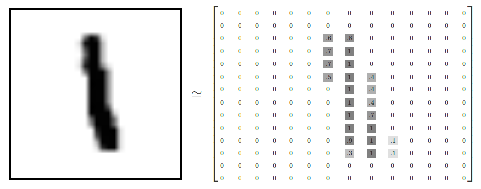
To make things easier on the learning process, it is typical to ignore color when possible, and instead examine grayscale representations of each pixel ranging from 0 (white) to 1 (black), and storing these values into a matrix with each pixel corresponding to each cell.
Here's a pictorial representation of the above image decomposition from Google's Tensorflow, a popularly used toolkit that we'll hint at again later:
Some classical datasets are publically available for "baselining" different ML approaches, and hand-written digits are no different:
The MNIST (Modified National Institute of Standards and Technology) Database of Handwritten Digits containts centered, grayscaled, and otherwise standardized 28 x 28 pixel images of hand-written digits, and can be found here.
So OK, we have our images in-hand, we can grayscale them to avoid the trouble of having to deal with different colors (which creates an even harder learning problem)... what now?
Is there any obvious way to get an algorithm to perform this task?
Note that even in small images that are 28 x 28 pixels, that's 784 features to consider, each which can hold continuous values between 0 and 1!
Brainstorm: any thoughts for how to tackle this classification problem?
Perhaps we can try to take those primitive features (pixels) and transform them into higher-order features like edges and shapes (e.g., an 8 is kind of a composite of two circles)
Easier said than done! It's challenging to think of a basis for such a procedure...
...except we do it without effort all the time (you're doing it just be reading these notes)!
Indeed, the fields of neuro- and cognitive science have long tackled this very problem but from the biological side... perhaps they have some light to shed on the situation!
Influences from Neuroscience: The Visual System
Since we're taking a small detour into neuroscience, we should just be aware of the target for our current classification task: the human visual system!
The visual system is a staggeringly complex neural pathway starting at the eye's retina (input) whose signals travel through the optic nerve, and eventually reach the primary visual cortex for processing.
As the signal travels from retina to cortex, different parts of the brain are responsible for extracting higher-order primitives from the visual input; for example, two areas in the visual cortex, V1 and V2, are thought to process edge, corner, and motion detection.
Here is a depiction of the various stages in human visual processing, and the various higher-order primitives that are output:

Note the merit of the way it works for us humans: large amounts of primitive input is delivered through the retina, but is then grouped and interpretted the farther down the pathway the signal travels.
This seems like a pretty good system to emulate, especially if we have this notion of grouping high-dimensional features into more and more specific (and therefore, lower-dimensional) ones, e.g.:
Rod cells in retina respond to light (or more accurately, absence of light, like pixels in image) to form primitive visual input.
Signal is propagated to V1 area of visual cortex to detect lines and edges of figures in visual field.
Inferior-temporal cortex detects larger shapes from V1's detected lines and edges.
Steps like the above form a hierarchical model of object recognition moving from lower-order primitive inputs to higher-order object recognition.
In ML, this is a special case of a particular field of study known as dimensionality reduction, wherein high-dimensional inputs (like pixels) are reduced to smaller, higher-order processing components (like lines and edges), which are easier to perform learning with.
Artificial Neural Networks
Given the neuroscientific background above, let's now revisit our image classification problem...
[Q1] What features \(f(x)\) would we want to extract for our image \(x\) in the MNIST dataset above? How would we go about extracting those that?
Hell if I know! Ideally we'd be able to take the individual pixels of the image, \(x\), and then look at the lines and shapes they formed, but the mechanics for doing that seem really messy and hard to code by hand!
Intuition 1: features on complex tasks are hard to extract top-down... so why not try to learn them from the training set alongside the classification task?
The second issue somewhat stems from the above:
[Q2] If we don't know what the features are for an ML task, why might logistic regression's linear decision boundary be a problem?
The relationship between the unknown features and class may be highly nonlinear! The simplifying assumption of linearity that allowed LR a lot of generalizability may not apply to all scenarios.
Take, for example, the XOR(input1, input2) = output function, which, if we consider a binary classification task where the output is some assigned
class, we'd have one heck of a time using linear classifiers to fit.
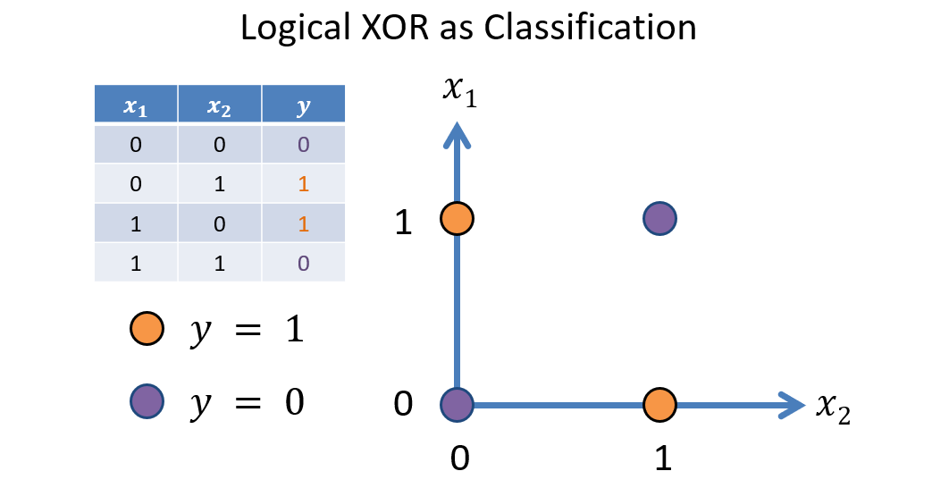
Intuition 2: some classification tasks may require solutions that possess a nonlinear decision boundary.
XOR is an artificial example of this intuition, but the following is not hard to imagine:
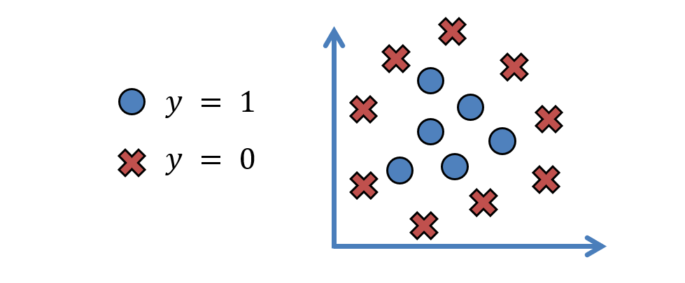
The above problems (when it's too hard to design features from the top-down and we have no guarantees about linear separability) distinguishes traditional machine learning (like we've been doing) from deep learning, in which an artificial neural network is used to learn the features for us!
The way we visualize this difference is as follows:
Our Multi-class Logistic Regression is a special case of neural network structured as follows:
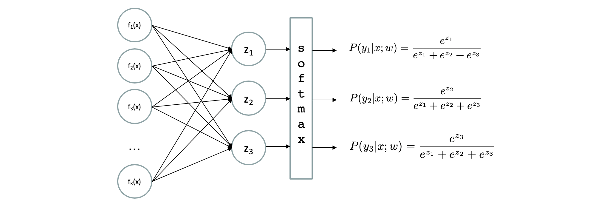
Modified from Berkeley's AI materials, with permission.
Idea: *on top of* learning the weights mapping each feature insofar as they predict each class, treat each feature \(f_i(x)\) as its own learning task!
If we think of Logistic Regression as a single neuron / unit, then implementing the above means stringing many neurons together to make a network.
A Feed-Forward Neural Network expands the Logistic Regression architecture by trying to approximate the feature extractor, \(f(x)\) with the following changes:
We have an input layer (leftmost) that is the raw-input (pixels of an image, words from an email, etc.)
We have an output layer (rightmost) that consists of one output for each class \(y \in Y\); these would be the softmax likelihoods in our logistic regression examples.
We have 1 or more hidden layers (between the above) used to learn *some* features from the raw input!
Depicted:
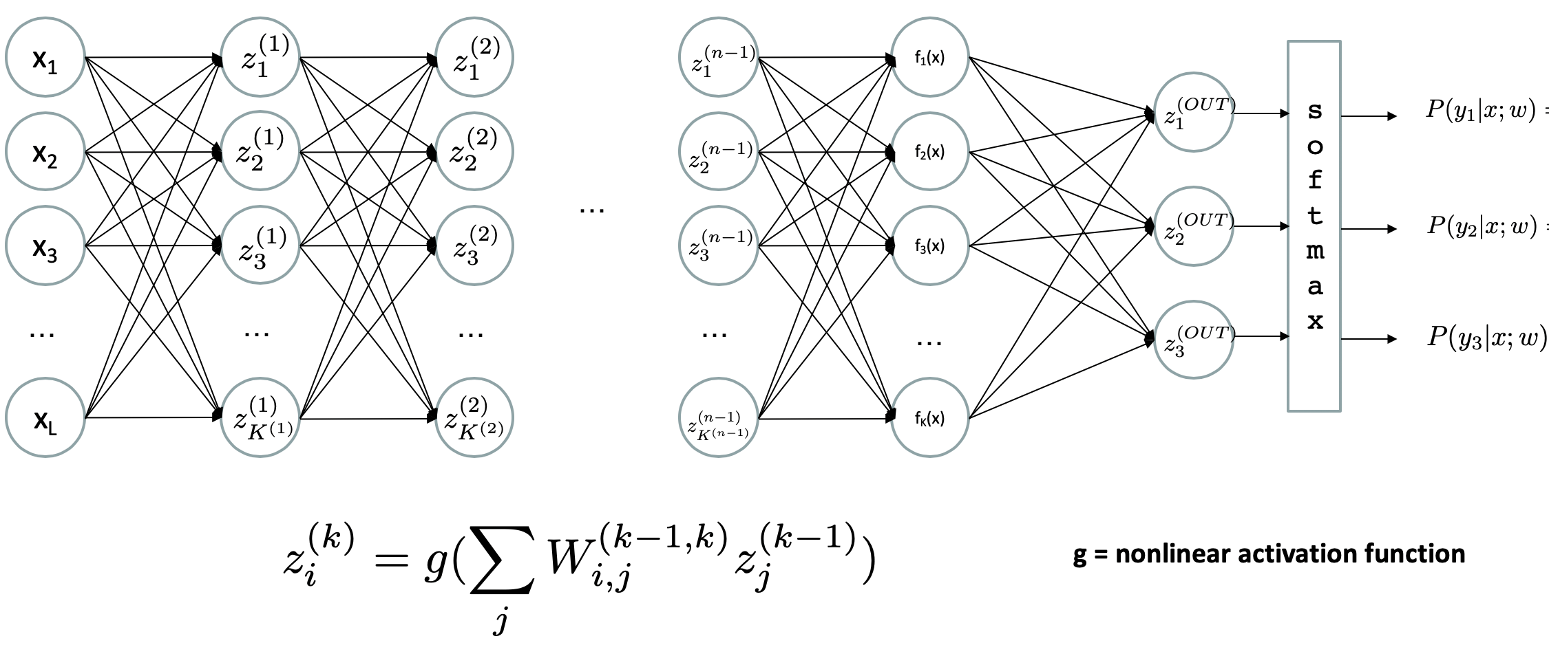
Modified from Berkeley's AI materials, with permission.
In particular, what's displayed above:
The input layer is left-most, output layer is right-most, and several hidden layers are in-between.
Each Circle above represents a single neuron with its own activation function and set of weighted inputs, just like we've been seeing with Logistic Regression.
This depiction is that of a "dense" neural network in which every unit / neuron in layer \(k+1\) is connected to each unit in the previous layer \(k\).
Feed-forward Neural Networks are once more parameterized by the weights between each unit at each layer, but before even thinking about the weights, there are a number of choices that the network designer has to make:
Structure Choice 1: how many hidden layers are included, how many neurons / units are within each, and how are the hidden layers connected to one another?
There is a wealth of literature that specifies different network structures for different tasks, e.g., more complex vision tasks using a Convolutional Neural Network where special convolution and pooling layers group nearby pixels from an input image.
Rule of thumb: most simpler classification tasks can be solved using a single hidden layer, but the more layers and units that are included, the more data the network takes to train, and the less generalizable / interpretable it becomes.
Structure Choice 2: what activation functions belong to each unit at each hidden layer.
There are many different activation functions out there, and the literature is still evolving on which are best to use under what circumstances; here are a few:
In order to be useful for addressing our intuitions above and some later qualities of neural network learning, any activation function we choose must be (1) differentiable (think: gradient descent) and most are (2) nonlinear.
This makes Neural Networks a linear-combination of non-linear activations, and thus a form of generalized, nonlinear function approximation.
Suppose we have the following tiny feed-forward neural network with:
2 inputs, \(\{x_1, x_2\}\)
1 hidden layer with 2 neurons / units, \(\{z_1, z_2\}\)
A single output neuron, \(y_1\)
Weights for each input into a neuron along the input edges, as depicted in the following diagram
Sigmoid activations at each non-input neuron: \(z_i = \sigma(in_i) = \frac{1}{1+e^{in_i}}\) where \(in_i\) is the weighted sum of outputs from the previous layer (ignore any "bias" terms for simplicity).
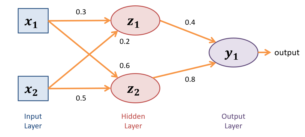
Suppose for a single sample we have \(\{x_1 = 1, x_2 = 2\}\); determine the output of this network at \(y_1\), as might be the likelihood of the positive class for a binary classification task?
Computing Inputs \(\rightarrow\) Hidden Layer:
\begin{eqnarray} z_1 &=& \sigma(in_{z_1}) = \sigma(1 * 0.3 + 2 * 0.2) = \frac{1}{1+e^{-0.7}} \approx 0.67 \\ z_2 &=& \sigma(in_{z_2}) = \sigma(1 * 0.6 + 2 * 0.5) = \frac{1}{1+e^{-1.6}} \approx 0.83 \\ \end{eqnarray}As such, these two outputs from \(z_1, z_2\) are then fed-forward to units / neurons in the next layer. In this case, that next layer happens to be the output with a single unit, but we could scale this to additional hidden layers or additional output units depending on the network architecture.
Computing Hidden \(\rightarrow\) Output Layer:
\begin{eqnarray} y_1 &=& \sigma(in_{y_1}) = \sigma(0.67 * 0.4 + 0.83 * 0.8) = \frac{1}{1+e^{-0.932}} \approx 0.72 \\ \end{eqnarray}Neural Network Learning
There's a lot to say about how learning works in a neural network -- here's a handwavy explanation and you can go on to study more in specialized deep learning classes!
Just as with logistic regression, learning in neural networks is to determine the best set of weights by the same maximum-likelihood metric AFTER the network's structure has been fixed (i.e., # of hidden layers and units etc. have been decided already).
Neural network learning works the same as in Logistic Regression, but with one catch: the blame for any discrepancies at the output layer get propagated back to earlier layers whose activations were responsible for the errors.
There's a wonderful video series that I can't recommend enough that will tell us all we want to know about learning in neural networks -- at least at a high enough level required for the end of this class! Take a look:
Neural Network Gradient Descent (Watch up to 11:17)
For completeness, here is the full back-propagation algorithm as detailed by your textbook:
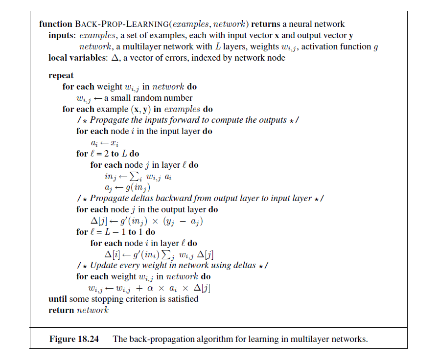
This brief introduction to network learning is yet another tip of the iceberg; there have been thousands and thousands of papers written on network tuning, but having these fundamentals will begin your long, rewarding journey!
Neural Network Summary
Pros |
Cons |
|---|---|
Can be used to create high-performing classifiers on complex problems, even when the features are unknown and optimal decision boundary non-linear. |
Require huge amounts of data to train successfully. |
Can involve little to no feature-engineering, though data preparation is still important. |
Once trained, the underlying model is not particularly interpretable; difficult to say why it works or doesn't, and features don't get "learned" in a human-intuitive way. |
Many libraries that support flexible Neural Network design and training, including |
The job of a NN is to overfit to its training data due to its ability to learn nonlinear decision boundaries, so generalizability is often very difficult. |
And there you have it! NNs in a nutshell.
Next week, we'll examine a fun in-class activity surrounding them.
Supervised Learning Summary
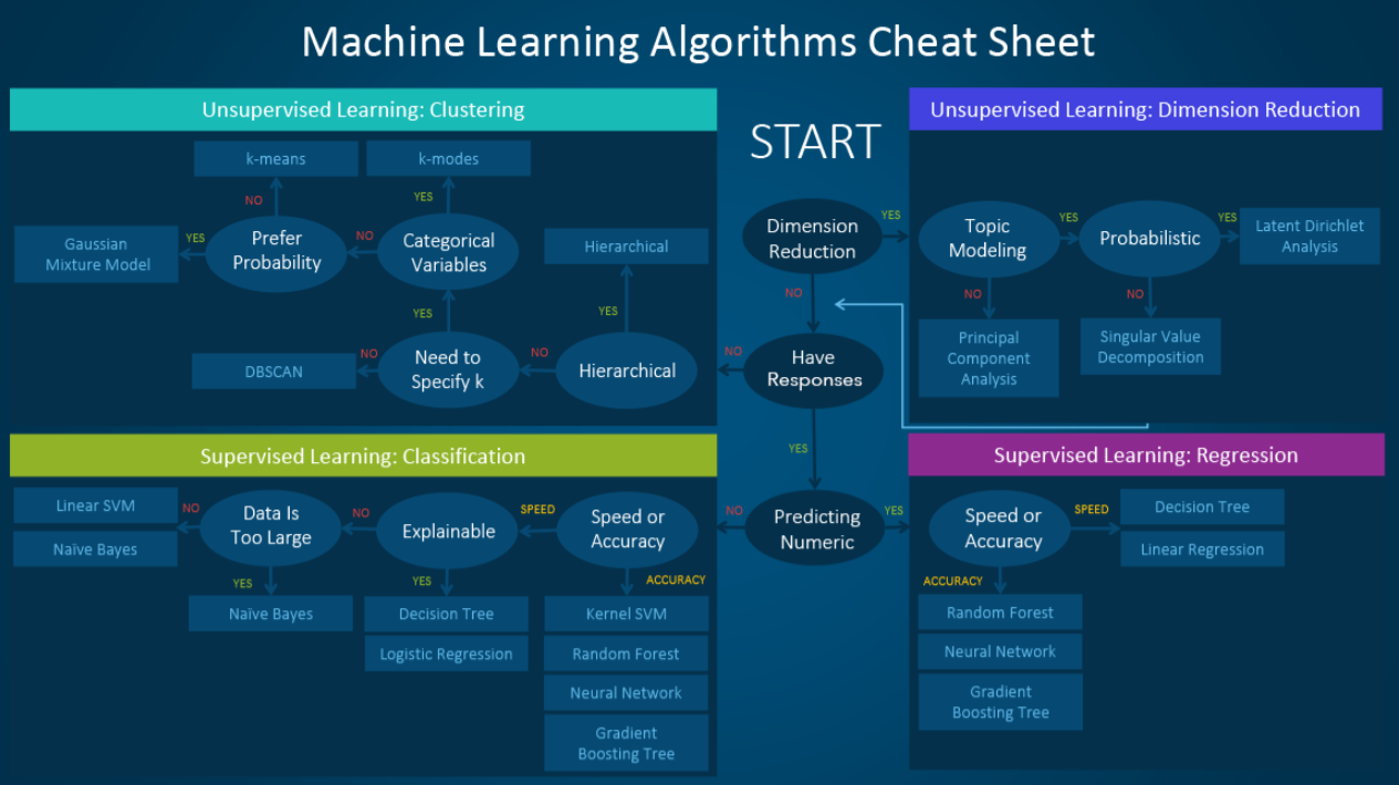
So now that we've seen a variety of different models for supervised learning... let's take a second to look at the big picture.
Here's a very brisk summary of the models we've learned about:
Naive Bayes Classifier: simple, easy to learn, can handle small AND huge amounts of data alike, works well for classification of small problems.
Logistic Regression: also simple, takes a bit longer to learn and requires a bit more data, but more interpretable since we get likelihood outputs and weights that correspond to different features -- can also weight different features differently.
Neural Networks: require huge amounts of data, usually overfit, highly uninterpretable, but very powerful and don't always require programmers to engineer features.
Notes on the above:
We only got to explore the lower left (and really, the lower right as well though we didn't see these types of prediction problems -- we'll see more in Cognitive Systems!), and there are even more models outside of those listed here to explore!
If you have time, you should really investigate Decision Trees and Random Forests / Ensemble Methods -- they're another very popular method for supervised learning, and there's more info in our textbook (same with Support Vector Machines [SVMs]).
That, my friends, is all that we have time for in this already bloated semester -- how time flies!
I hope you enjoyed the journey and should be proud of how far you've come learning this dense, but wonderous, material. The world is your oyster, go forth and explore what excites you most from the brief exposure we got together this year!