Quantifying Uncertainty
Someone once made a very astute observation when we were discussing our propositional logic example with rain making the sidewalk wet:
They asked, "We have these general rules that the sidewalk will always be wet if it's raining, but what if the sidewalk is covered by a tree during the storm?"
Clearly there are exceptions to our general rules, and it's often difficult to represent the infinite number of exceptions that could happen with propositional logic.
Let's consider a motivating problem.
Motivating Problem
Suppose we are designing Forney Industries' Solicitorbot 5000, which sells products door-to-door but must decide which houses to visit to maximize its sales.
To imbue Solicitorbot with some logic, suppose we implement a simple propositional logic system so that it doesn't visit houses that won't lead to sales:
  # Let L = whether or not the house's lights are on
  # Let H = whether or not someone is home
  KB =
     # "If the lights are off, no one is home"
     1. ¬L => ¬H
     # "A house's lights are off"
     2. ¬L
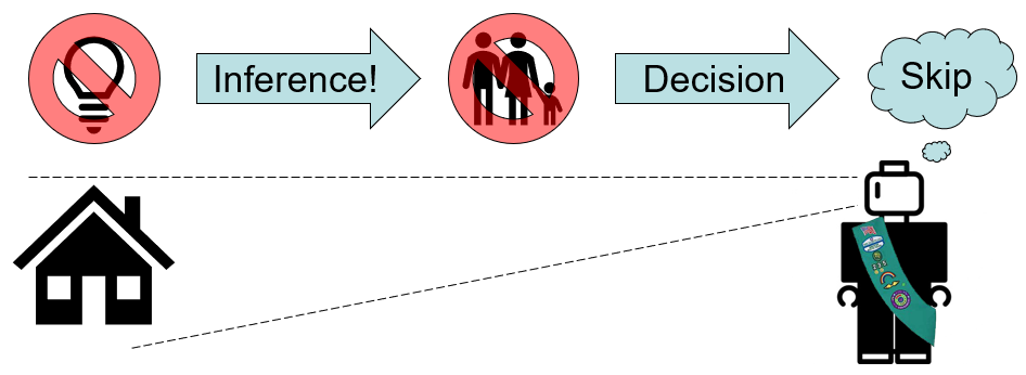
Plainly, if Solicitorbot sees the lights of a house off, it should skip that house (according to our rule-based system).
However, we can start to see that there might be some cracks in this reasoning system...
What are some exceptions to the \(\lnot L \Rightarrow \lnot H\) rule above? How would we repair for these exceptions in propositional logic KBs?
Example exceptions might be:
Whether or not the residents' shades are down (S)
Whether or not the lights are on a timer (T)
etc. etc.
We would repair for these by adding conditions to the rule's premise, a la: $$(\lnot L \land \lnot S \land \lnot T \land ...) \Rightarrow \lnot H$$
Of course, we want our reasoning system to remain faithful to reality, so considering these exceptions would be necessary for our KB's representation to match the state of the world it is representing.
There are many issues with our method of repairing for exceptions above. What are they?
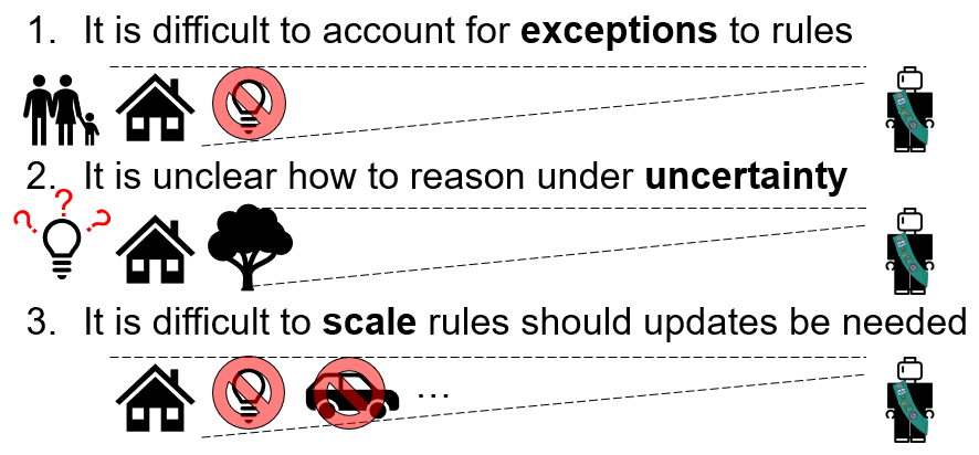
Three primary shortcomings:
The list of rules describing when the residents are home is incomplete; e.g., perhaps whether or not someone's car is in the driveway is a better indication that they are home than their lights.
Since propositions are simply implementations of boolean logic, we have no means of representing chance / uncertainty; e.g., our agent cannot determine whether or not the lights are on because a tree is blocking the house from the street.
The rule for whether or not someone is home does not easily scale with exceptions; e.g., we listed only 2 of the many many reasons why someone may or may not be home based on their house's light status.
Pictorially:
Suggest some ways to address the shortcomings of propositional logic.
Whatever your answers to the above, the approach that followed historically from rule-based reasoning systems was born from acknowledging the following:
We cannot model every single exception to every single rule in any sort of realistic fashion.
Instead, however, we can summarize exceptions by what is likely to happen in a given scenario.
At the core of this approach: the more our agents know about their environments, the less uncertainty.
Uncertainty about an environment arises in imperfect information problems wherein (for example) the agent has partial sensor information, ignorance of the rules of the environment, or the environment is fundamentally nondeterministic.
The problem with uncertainty is that, even though the agent does not have "all the facts," it is still expected to choose as optimally as possible.
And thus, the domain of probabilistic reasoning was born.
Probabilistic reasoning models uncertainty in the environment in a parsimonious, statistical representation that then allows the agent to act as best as it can with the information it has available.
Understanding probabilistic logic requires, unsurprisingly, that we understand something about probability theory, and the symbolic representation of how we model uncertainty.
Introduction to Probability Theory
The beginnings of probability theory do not far diverge from our beginnings of propositional logic.
In propositional logic, how did we think about the truth of a sentence in all possibilities of our propositions?
We examined that sentence \(\alpha\)'s models in a truth table!
So returning to our Solicitorbot design, we would decompose all possible instantiations of propositions into "worlds" with certain interpretations:
World |
L |
H |
Interpretation |
|---|---|---|---|
\(w_0\) |
F |
F |
The lights are off and no one is home |
\(w_1\) |
F |
T |
The lights are off but someone IS home (hiding from Solicitorbot?) |
\(w_2\) |
T |
F |
The lights are on but no one is home (wasteful!) |
\(w_3\) |
T |
T |
The lights are on and someone IS home |
Are any of the above worlds impossible? Are some more probable than others?
We can likely generate an explanation for any of the above, yet, some are certainly more likely than others (e.g., it is probably rare that the house's lights are off but someone is home).
Just as propositional logic allowed us to make claims about the set of possible worlds in an environment using logical sentences, in probabilistic logic, we will instead reason over the space of probabilities that we are in each world.
Probabilistic Logic Syntax
Just as we had the syntax of propositional sentences, so too must we learn how to discuss quantities using probability theory.
Let's juxtapose propositional logic with probabilistic logic below:
Propositional Entity |
Probabilistic Analog |
Probabilistic Syntax |
Interpretation |
|---|---|---|---|
Proposition |
Event / Random Variable |
Capitalized letters, words |
|
Values |
Values |
Lowercase letters, words. |
|
Truth Table |
Probability Distribution |
\(P(A \land B \land C \land ...) = P(A, B, C, ...)\) for distribution \(P\) over variables \(A, B, C, ...\). |
|
Models |
Probability Value |
\(P(A = a, B = b, C = c) = P(a, b, c)\) for distribution \(P\) over values \(a, b, c\). |
|
Let's look at an example of the above!
For discrete variables, probability distributions are defined tabularly, since every world (i.e., instantiation of variables) will be assigned some probability. The fully-specified table that provides this mapping for all variables in the model is called the joint probability table.
Joint probability tables, specified via \(P(A \land B \land C \land ...) = P(A, B, C, ...)\) define the likelihood of seeing event \(A \land B \land C \land ...\) for all variables and their associated values.
These distributions are termed "joint" because they describe the probability of seeing a particular instantiation of variables together.
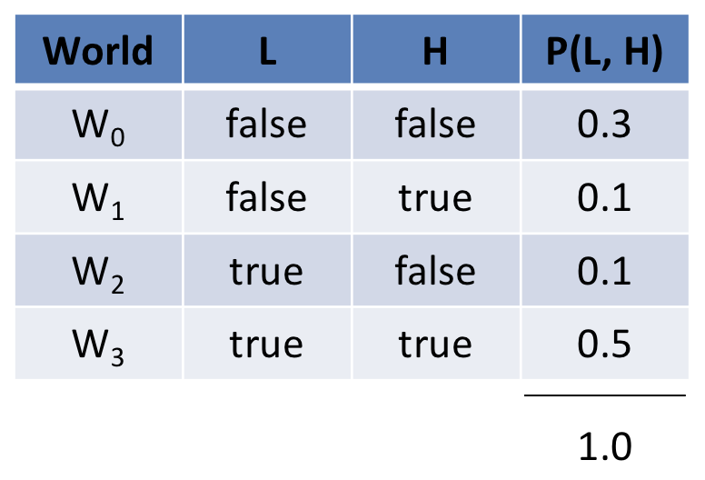
Observe the following joint distribution over our Solicitorbot example's variables: L (whether or not a house's lights are on) and H (whether anyone is home).
World |
L |
H |
\(P(L, H) = P(L \land H)\) |
|---|---|---|---|
\(w_0\) |
false |
false |
\(P(L = false, H = false) = 0.30\) |
\(w_1\) |
false |
true |
\(P(L = false, H = true) = 0.10\) |
\(w_2\) |
true |
false |
\(P(L = true, H = false) = 0.10\) |
\(w_3\) |
true |
true |
\(P(L = true, H = true) = 0.50\) |
Note: Joint Probability Tables describe the probability of seeing the variable instantiations in each world without / before any other evidence.
Harkening back to propositional logic, we might think of this as the state of the knowledgebase before any facts are gathered.
In other words, they describe the raw probability values of every world.
Reasonably, you might ask, where do these probability values come from?
Typically, from (1) large datasets that have been gathered observationally/experimentally, (2) expert opinions, and (3) an agent's experience (i.e., updated based on the agent's experiential history).
Now that we've seen these tables, we should be formal and understand some of their axiomatic properties (the properties that are true by definition).
Axiomatic Properties of Probability Theory
There are only a few axioms that constrain probability theory as amounting from the formalization of a joint distribution:
Probability Value Range: All probability values assigned to any given world \(w\) must range between 0 (impossible) and 1 (certain), inclusively: $$0 \le P(w) \le 1$$
The sum of all probability values in worlds \(w\) that are possible must sum to 1: $$\sum_w P(w) = 1$$
Law of Total Probability: The probability of any subset of variables, \(\alpha\), is the sum of every possible world \(w\) that in that subset's models: $$P(\alpha) = \sum_{w \in M(\alpha)} P(w)$$
We can quickly verify that the first two axioms are met by our Solicitorbot joint probability table above, but consider the following:
What is the raw probability (i.e., the prior) that someone is home? In other words, what is \(P(H = true)\)?
Using the third axiom above, we see that: $$P(H = true) = \sum_{w \in M(H = true)} = P(w_1) + P(w_3) = 0.60$$
Probabilistic Semantics
Just as we can define the language to denote uncertainty (i.e., the syntax), we should think about just what we're saying when we do: let's dive into the semantics.
To motivate this exploration, consider why we are reasoning in the domain of probabilities to begin with.
The power of probabilistic reasoning is not simply captured in its ability to assign chance to different "worlds," but rather, represents an agent's beliefs about the likelihood of each world that can be updated as information is gathered.
We've seen this capacity for an intelligent agent in propositional logic, but now we need to translate it to the domain of probabilistic logic.
Probabilistic Inference is the ability to reason over probabilities of likely worlds given evidence that is observed about the environment; this is sometimes called Bayesian Inference.
If an agent believes that some worlds are more likely than others, it may modify its behavior accordingly.
Reconsider our Solicitorbot from earlier, in which we assigned probability values to all possible worlds partitioned on \(L\) (whether or not a house's lights are on) and \(H\) (whether or not someone's home).
The joint probability distribution encoded the raw chances of seeing a particular instantiation of variables without assuming that our agent knows any other information about the environment.
World |
L |
H |
\(P(L, H) = P(L \land H)\) |
|---|---|---|---|
\(w_0\) |
false |
false |
\(P(L = false, H = false) = 0.30\) |
\(w_1\) |
false |
true |
\(P(L = false, H = true) = 0.10\) |
\(w_2\) |
true |
false |
\(P(L = true, H = false) = 0.10\) |
\(w_3\) |
true |
true |
\(P(L = true, H = true) = 0.50\) |
Just as in propositional logic, we added knowledge to our KBs whenever observations were gathered via the tell operation. In probabilistic logic, we add knowledge to our system by restricting
the set of possible worlds to be consistent with observed evidence.
Updating our knowledge about the environment was important for making inferences in the same way that in probabilistic reasoning, we should update our beliefs about the chances of worlds in our environment.
Looking at the above, suppose our agent observed that a house's lights are on (i.e., \(L = true\)). How (if at all) should this observation change the probability that someone is home?
We would expect, looking at worlds \(w_2, w_3\), that observing a house's lights on would increase the agent's belief that someone is home.
This intuition is well-founded, but what we now need is a means of formalizing our intuition that is aligned with the syntax of probabilistic reasoning.
In other words, we need to establish the rules that govern how we transform knowledge about the joint distribution and put it into the context of observed evidence about the environment.
Conditional Distributions
Returning to our joint distribution (hey, suddenly it looks like something from a PowerPoint, go figure >_> <_<)
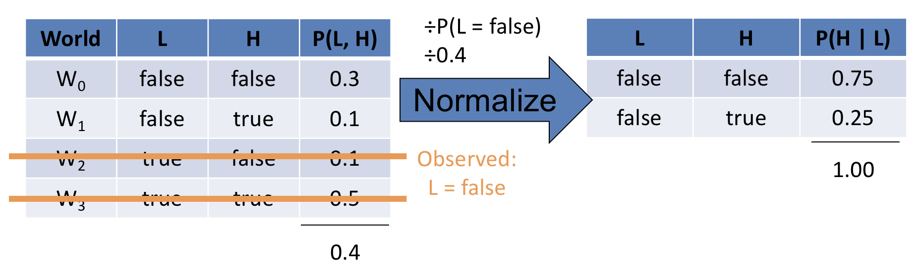
Suppose our agent observes that a house's lights are off (i.e., \(L = false\)), which worlds above become impossible, and why?
\(w_2, w_3\) become impossible because they conflict with the observed evidence.
Formally, Observations / Evidence constrain the set of possible worlds in probabilistic reasoning by assigning a probability of 0 to worlds that are inconsistent with the evidence.
The observation that \(L = false\) thus "zeros out" rows of the joint distribution table that are inconsistent with the evidence.
Thus, we are left with the following restriction imposed on the joint:
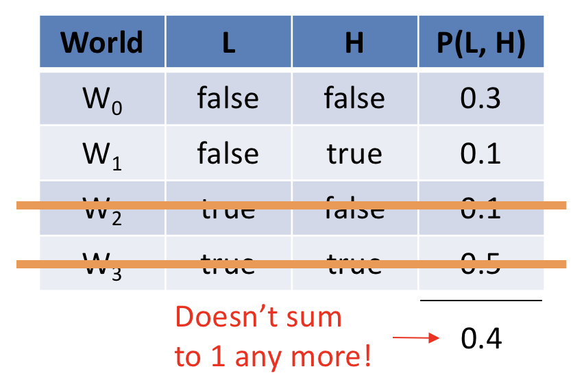
Note, however, that we have violated one of our axioms of probability theory: that the sum of all possible worlds (even under some observed evidence) shall always sum to 1!
How can we repair this violation of the axiom to be left with a legal probability distribution?
Normalize the remaining worlds \(w\) that are consistent with the evidence \(e\) by: $$\frac{P(w)}{P(e)}$$
Normalizing joint values after accounting for observed evidence leaves us with what is known as a conditional distribution.
A conditional probability distribution specifies the probability of some query variables \(Q\) given observed evidence \(E=e\), is expressed: $$P(Q | E=e) = P(Q | e)$$
Some notes on that... notation:
The bar | separating \(Q\) and \(E=e\) in \(P(Q | E=e)\) is known as the "conditioning bar" and is read as "given", e.g., "The likelihood of Q given E=e"
The query variables are what still have some likelihood attached to them, but now under the known context of the evidence (assumed to be witnessed with certainty, which is why they're assigned \(E=e\))
Putting our observation from above to a name and an equation, we see one of the most important rules in probability calculus:
Probabilistic Logic Tool - Conditioning: for any two sets of queries and evidence we thus have: $$P(Q | e) = \frac{P(Q, e)}{P(e)} = \frac{\text{joint prob of \{Q, e\}}}{\text{prob. of \{e\}}}$$
Applying this tool to our problem above, we see that we can obtain the conditional distribution \(P(H | L)\) as follows:
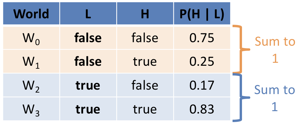
Repeating conditioning for the case where \(L = true\) gives us the following conditional probability table (CPT):
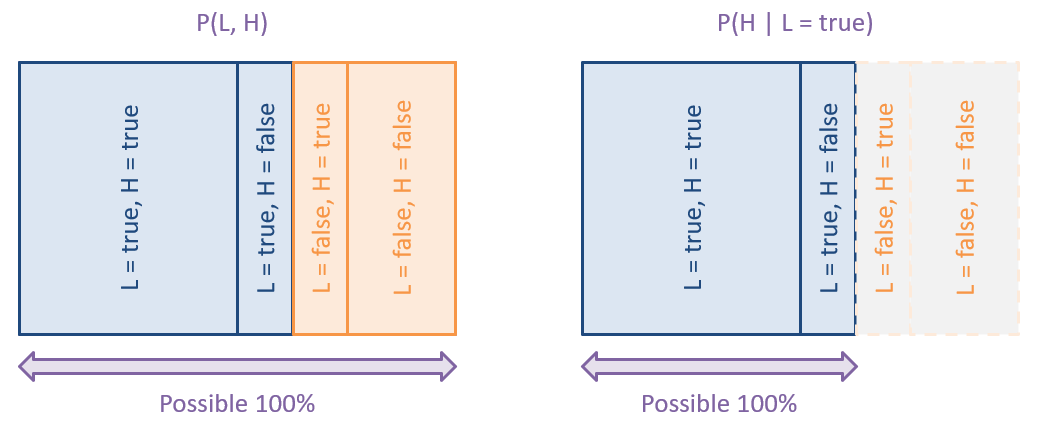
To visualize conditioning, consider the following diagram in which we constrain the proportion of the original probability mass based on what worlds are still possible:
Given the CPT above, and assuming our Solicitorbot wishes to visit only houses where someone is home, should it visit a house whose lights it observes are off? (i.e., \(L = false\))
No! It is more likely that no one is home when it is observed that the lights are off (\(P(H = false | L = false) = 0.75 > P(H = true | L = false) = 0.25\))
Note also the flexibility of probabilistic logic in this case: our agent will not be surprised if no one is home when the lights are on, since it is only a higher probability, but not a certainty that lights => being home.
As such, conditioning satisfies two of the issues that we experienced with propositional logic: the ability to gracefully deal with exceptions and uncertainty.
We'll address the third issue, scalability, in the next section and lecture...
Independence
Suppose we wanted to improve the accuracy of our Solicitorbot to take more features into consideration that would indicate whether or not someone is home.
Suppose we added a new variable, \(C\), to the system representing whether or not Solicitorbot hears a *cacophony* (flexing our vocab too) within the house (that's a loud, jarring noise).
Note: in propositional logic, this would be a cumbersome task: we would have to update every rule that would relevantly mention \(C\).
In probabilistic logic, however, this addition expands the joint distribution such that we have:
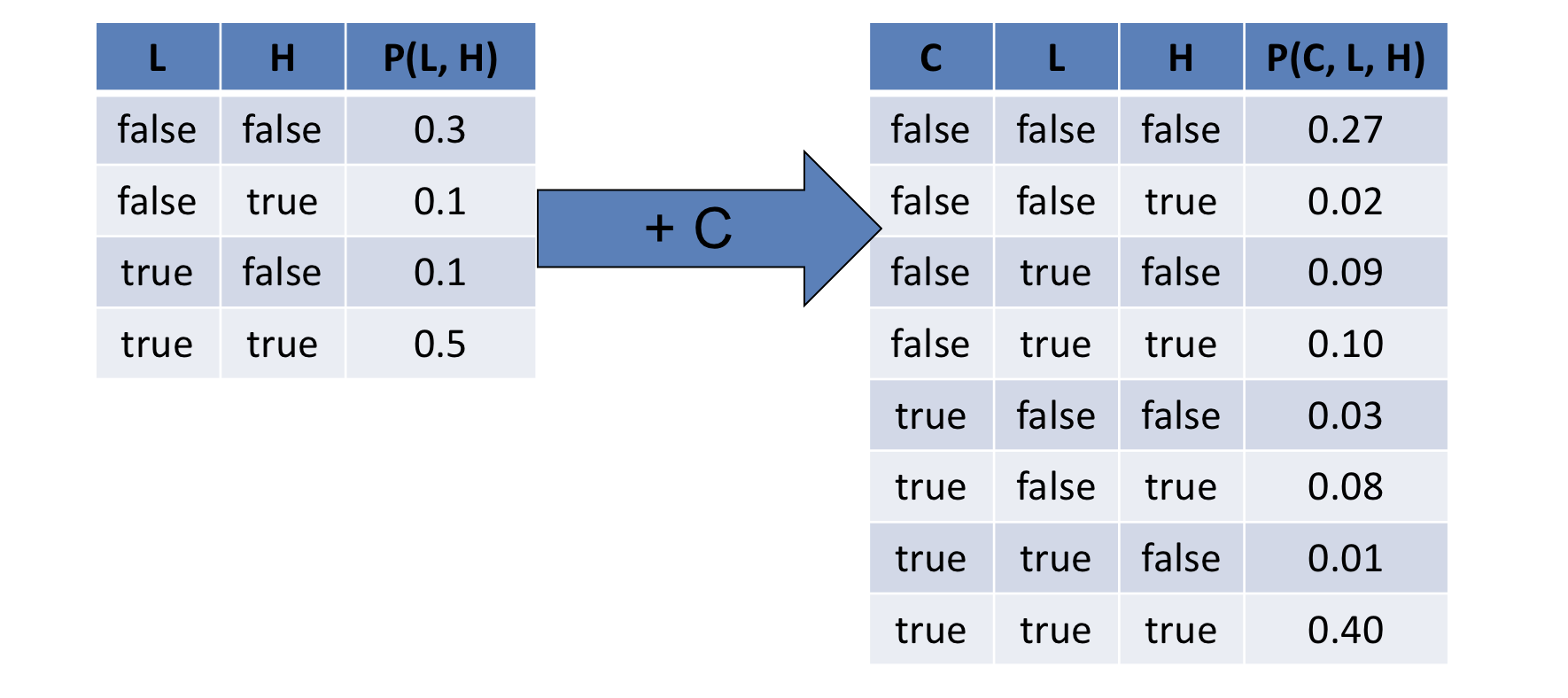
Given that our random variables need not be binary, how many rows will there be in the joint distribution?
The product of every variable \(V\) cardinality: $$\prod_{i} |V_i|$$
It would seem that we have some growing pains again!
In the same way that the number of possible worlds grew exponentially in propositional logic truth tables, we can see that the joint distribution will grow very quickly in probabilistic logic as well.
So, what can we do to ameliorate this growth?
Factoring the Joint Distribution
Suppose, instead of storing every row of the joint distribution, we were about to factor it into smaller sub-components.
To do so, we'll need a means of "chopping it up," and to help us with this task is a nice attribute from probability theory that we'll motivate next.
Suppose we roll two, fair, 6-sided die: \(A, B\). Will the outcome of \(A\) tell me anything about the outcome of \(B\)? In other words, does treating \(A\) as evidence update my beliefs about \(B\)?

No! Knowing the outcome of \(A\) tells me nothing about the outcome of \(B\) since they are two dice rolls with nothing to do with each other.
If the evidence of \(A\) tells us nothing about \(B\), what can be said about \(P(B|A)\)?
If \(A\) is irrelevant to \(B\), then: \(P(B|A) = P(B)\)?
Two variables \(A, B\) are said to be independent, written \(A \indep B\), if and only if the following holds: $$A \indep B \Leftrightarrow P(A | B) = P(A) \Leftrightarrow P(B | A) = P(B)~\forall~a \in A, b \in B$$
In other words, independence is a measure of relevance between variables.
We only want our agent's observed evidence to change its beliefs about those variables for which the evidence is relevant!
So, how does this help us factor the joint distribution? Well, let's consider our dice again...
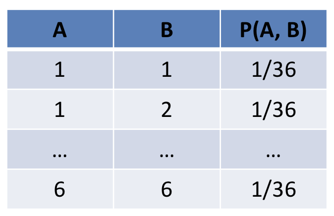
What would the joint probability distribution / table look like for two independent, fair, 6-sided dice rolls for dice \(A, B\)? How many rows would it have?
The table would have 36 rows (1 for each combination of values for \(A, B\)) and look like:
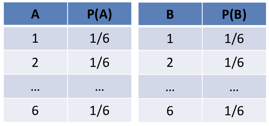
Now, consider the probability distributions over each dice individually; what would the distribution tables for \(P(A), P(B)\) look like, and how many rows would they have?
They would each have 6 rows a piece (for a total of 12) and look like:
How, then, can we relate the joint distribution of two independent variables \(A, B\) to their individual prior probability distributions \(P(A), P(B)\)?
If \(A \indep B\) then: \(P(A, B) = P(A) * P(B)\)
And thus we have yet another tool at our disposal:
Probabilistic Logic Tool - Joint Independence Factoring: for two variables \(A, B\): $$A \indep B \Leftrightarrow P(A, B) = P(A) P(B)$$
How does this help us "shrink" our joint distribution? Consider the dice joint with 36 rows.
We can derive any row of the joint by multiplying the priors. As such, we need only store 12 rows rather than 36.
Brilliant! So it would seem that identifying independence relationships between variables in our system leads to a more parsimonious storage of the joint distribution, from which we can answer interesting queries of probabilistic inference.
However, there's a bit of a wrench to throw in the gears...
Conditional Dependence
Returning to the 2 fair die problem, suppose we add another variable into the system: \(S\), representing the sum of the individual dice rolls, i.e., \(S = A + B\)
We know that \(A \indep B\), but suppose I told you the outcome of \(A = 6\) and the sum of the dice rolls \(S = 7\). Does knowing about \(S, A\) change our belief about \(B\)?
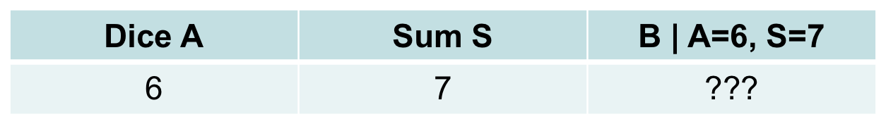
Yes! If I told you that \(A = 6\) and \(S = 7\), then you should infer that \(B = 1\).
Curiously, above we have a scenario wherein \((A \indep B)\) but \((A \not \indep B | S)\)
Two variables \(A, B\) can be made conditionally dependent or independent when given evidence of another set of variables \(C\).
This complicates our ability to shrink the joint distribution via factorization!
Summary
Using the joint distribution, we can compute the answer to any interesting probabilistic inference queries...
...BUT, the joint distribution grows exponentially every time we add another variable to the system...
...however, we can store the joint distribution more parsimoniously by exploiting independence relationships between variables...
...BUT, the possibility of independent variables made dependent by conditioning on another set of variables exists!
So, what do we do?!
Find out next time!