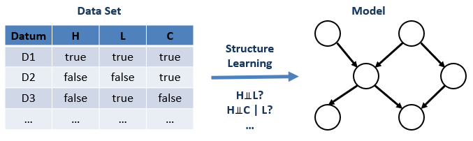
Structuring Independence
Last time, we saw that the Joint Probability Distribution provides all of the interesting information that we need to answer probabilistic queries about our environment.
When our agent does not have any observations about the system, we can consult the joint distribution itself, but when the agent does have observations, it can update its beliefs by consulting conditional probability distributions that (as we have )
The problem, however, was that the joint distribution grows exponentially with every variable that is considered, and so for any realistic reasoning system, we need a means to use the information of the joint without having to construct it or consult it explicitly.
This led us to consider independence relationships as ways to factor the joint distribution into pieces that we could more easily store and reason with.
So, reasonably, we must ask how we should structure or discover independence relationships such that we can then parsimoniously store the joint distribution.
Intuition of Structured Independence
To motivate the technique we'll use to structure independence relationships, we should develop some intuition behind what sort of data we have and why certain variables might be independent from one another.
Probability distributions (as we've been discussing) summarize associational / observational data such that a distribution denotes the witnessed correlations between variables in the system.
At what tier/layer of the causal hierarchy would we find this type of reasoning?
\(\mathcal{L}_1\), the associational! These associational likelihoods are little better than Pavlov's dog hearing that bell and salivating!
This is true of both joint and conditional distributions that we've seen thus far: when Solicitorbot sees that a house's lights are on, it is able to conclude that light status is positively correlated with someone being home, but no conclusion of causality is made.
Understanding that we are modeling correlations in our distributions gives us two pieces of intuition moving forward:
Independence Intuition 1: correlation does not imply causation.
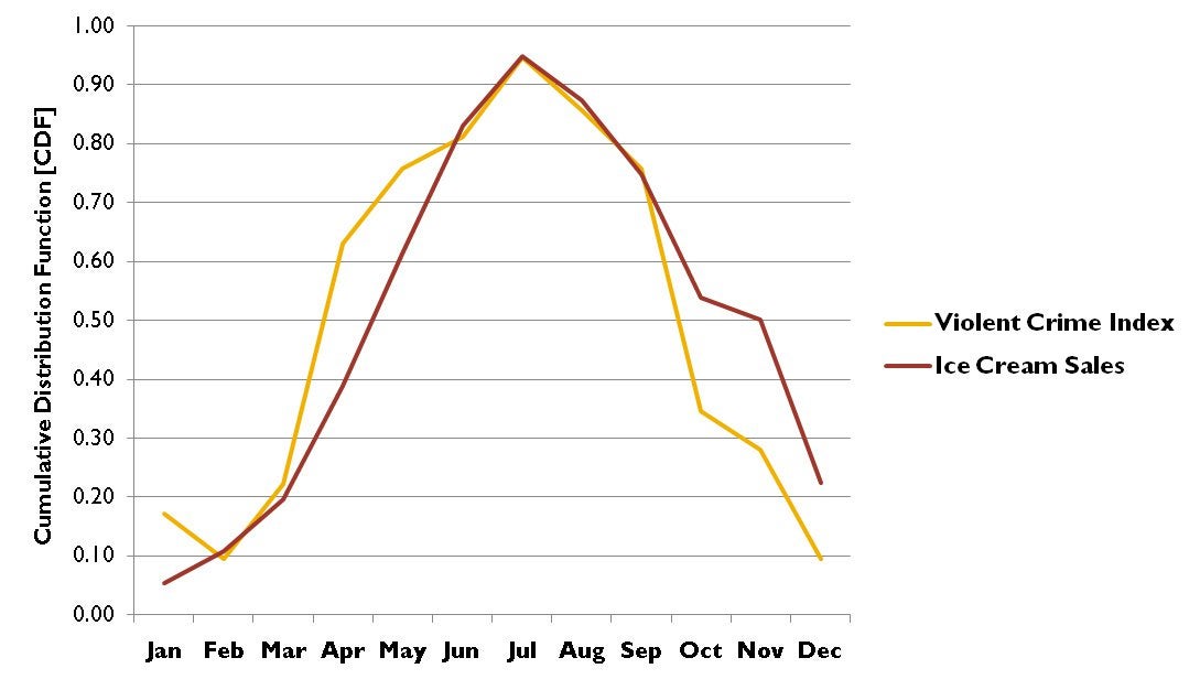
We, as adults, look at the above and laugh because it's plain to us that Ice Cream and Murder have no causal pathway between each other...
Which isn't to say we couldn't have a laugh or two trying to explain the above:
What are some causal explanations that might be attached to the graph above (Ice Cream Consumption vs. Murder Rates)?
Ice Cream Consumption (ICC) sends people into a murderous rage (ICC causes Murder).
Murderers enjoy a nice post-murder ice cream (Murder causes ICC).
A third variable (viz., heat during the different seasons) lead people to both ICC and be a little on-edge (Heat causes both ICC and Murder).
The fact that any one of these explanations could "fit" the data in terms of explaining the correlation means that we cannot claim a causal relationship between ICC and Murder rates *without* some other assumptions, like the background common-knowledge that, in randomized controlled experiments, ice cream did not lead to increase in participants' propensities to murder.
From this warning, we receive the second intuition about our relationships between variables:
Independence Intuition 2: Causation does typically imply correlation: (aka Common Cause Assumption) if two variables are correlated, and there is some causal story that explains their relationship, then either one causes the other, or there is a third set of variables that causes both.
In other words, if two variables happen to "change with each other" (i.e., covary) it might be that one causes the other, or we might lack information on the variables that were actually to blame for their relationship (i.e., we did not collect data on the other variables).
So, we can start to see why we might want to think about relationships of cause and effect that we *can* model in our system in the effort of helping us think about independence (seen shortly).
Independence Intuition 3: thinking about the possible causal relationships between variables in the system can help us to structure the independence and conditional independence relationships between them.
Structuring Causal Assumptions
In this part of the course, we will discuss how we (the programmer) and our agent view their environment as seen through the lens of a model of the environment.
In probabilistic reasoning, Model-based Methods attempt to structure relationships between variables to provide a simplified perspective of the environment that an agent can reason with.
Given our interest in discovering independence relationships between variables in our system through assumptions about causes and effects, can we consider a data-structure choice that may well model relationships of cause and effect?
A graph! In particular, a directed, acyclic graph [DAG] (since causes cannot, intuitively, lead to their own causes!)
This is precisely the modeling technique that we'll begin with in what are known as Bayesian Networks.
Bayesian Networks - Structure
Yes that's right, it's time we were put on...

That, of course, is a picture of Father Thomas Bayes, the one responsible for the probability theory that governs Bayesian Networks, photoshopped onto David Hasselhoff's body from the hit drama series Baywatch (1989).
Why are Bayesian Networks so deserving of this fanfare? Well, let's start by defining them:
A Bayesian Network is a data structure used in probabilistic reasoning to encode independence relationships between variables in the reasoning system, and is composed of:
Structure: a Directed Acyclic Graph (DAG) in which nodes are Variables and edges (intuitively) point from causes (parents) to their direct effects (children): $$[Cause] \rightarrow [Effect]$$
[!] While the above directionality helps us to think about the structure, sometimes the relationship is non-causal in Bayesian Networks, and an edge \(X \rightarrow Y\) simply means that \(X \not \indep Y\)
Probabilistic Semantics: conditional probability distributions (or tables, in the case of discrete variables, known as CPTs) associated with each node.
Just how we attain the structure and semantics of a Bayesian network will be the topic of today's discussion.
Bayesian Network Structure
The structure of a Bayesian Network focuses on how we include and direct edges between nodes in the graph, and decides the independence and conditional independence relationships expected in the data.
Let's return to our motivating example to see how we might intuitively structure a Bayesian Network's nodes and edges.
Modeling Solicitorbot
Consider our Solicitorbot example once more in which we have variables:
\(H\) whether or not someone is home
\(L\) whether or not the house's lights are on
\(C\) whether or not there is a cacophony detected in the house.
We'll start by intuiting how the relationships of cause and effect should be oriented in our model.
Using a DAG, how should we model the relationships of direct causes and effects between these three variables in our graph?
In other words, for each arrow below, should the arrow exist at all (indicating a direct causal influence) and if so, what should it's direction be?
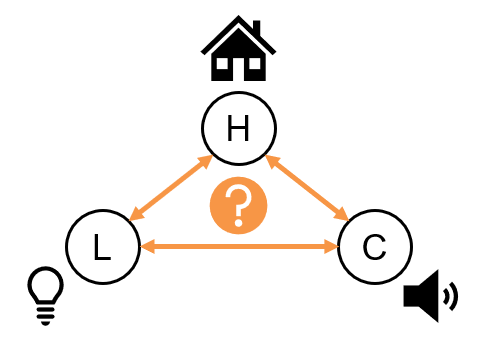
Intuitively, it is whether or not an individual is home that will be the *reason for* or *causal influence on* whether the lights or on or a car is in the driveway.
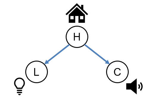
With this intuitively structured model of our Solicitorbot system in hand, let's consider what the model tells us about the independence relationships we should expect to find in our probability distributions.
Supposing \(L \leftarrow H \rightarrow C\), would we expect causes to be independent of their effects, i.e., should: $$H \indep L? \\ H \indep C?$$
No! We would expect that being home tells us something about the likelihood that the lights are on, and the likelihood that a car is in the driveway. So, \(H \not \indep L\) and \(H \not \indep C\)
Supposing \(L \leftarrow H \rightarrow C\), would we expect effects of a cause to be independent, i.e., should: $$L \indep C?$$
No! If a house's lights are on, then it's more likely that someone is home, which means that it's more likely that a car is in the driveway! As such, \(L \not \indep C\) since information about \(L\) gives us information about \(C\).
So we see that, without any other information, \(L, C\) are dependent -- they provide information about each other... but what if we know whether or not someone's home?
Does the information that they provide about each other add anything to the story?
Supposing \(L \leftarrow H \rightarrow C\), would we expect effects of a cause to be independent once we know the state of the cause, i.e., should: $$L \indep C~|~H?$$
Yes! If we know whether or not someone's home, then knowing whether or not the lights are on no longer tells us *anything more* about whether or not the car is in the driveway that we didn't already know from \(H\). As such \(L \indep C~|~H\)
In summary, the model structure that we currated entails the following independence relationships:
\(H \not \indep L\), \(H \not \indep C\), \(L \not \indep C\), \(L \indep C~|~H\)
If our model is correct, then we should witness these independence relationships hold from the data / joint distribution as well!
A reasonable next question is: in practice, where do Bayesian Networks come from? ("Where are Baye-s made?" typically a question for your parents [ok that one was a stretch]).
Model Sources
There are two main approaches for creating and then using Bayesian networks:
Top-down [Model -> Data]: start with a programmer-curated model and then interpret witnessed data through the model.
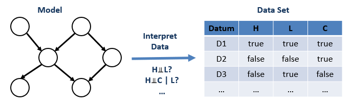
This is the approach that we used above!
We used our knowledge about the way the world works to intuit the relationships between variables, and could then use this model as a lens through which to interpret any data.
Bottom-up [Data -> Model]: start with data and attempt to learn the model (i.e., structure relationships between variables) based on witnessed independence relationships.
In the reverse, if we didn't want to start with a model, we could attempt to learn one by examining the independence relationships from the data.
Although we'll examine this method later, be warned that there are some practitioners who believe this to be a poor methodology for inferring causal relations because of the caveats of modeling associational data that we examined in the "Intuition" section above.
If we don't care whether or not the edge directions carry causal information, and just want to factor the joint distribution, this is still a good technique!
A network structure that implies the same independence relationships as are witnessed in the data are said to be faithful, which is a good property to aim for.
Disclaimer: the probabilistic inferences we gain from our models are only as good as the models are faithful to reality. Bad model in = bad inference out!
As such, the modeler must be able to defend their modeling choices on sound scientific principle or risk creating a faulty reasoning system.
Now that we've seen the structure of a Bayesian Network, and how to configure nodes and edges in the graph, let's take a look at their semantics.
Bayesian Networks - Semantics
The semantics of a Bayesian Network define the rules by which probabilistic queries can be made from the network.
Recall our original goal: to somehow "factor" the joint distribution using independence relationships.
Let's see how those independence relationships might aid us in this task.
Consider the joint distribution for the Solicitorbot example: \(P(H, L, C)\). We wish to use the independence relationship \(L \indep C~|~H\) to factor the joint distribution.
To accomplish this task, we'll need a couple of reminders:
Recall that the conditioning rule was that: $$P(Q | e) = \frac{P(Q, e)}{P(e)}$$ ...multiplying each side by \(P(e)\) we can solve for the joint in terms of the conditional distribution: $$P(Q, e) = P(Q | e)P(e)$$
This simple algebraic manipulation of the conditioning rule also bears an intuitive interpretation: $$\begin{eqnarray} P(Q, e) &=& P(Q | e)P(e) \\ \{\text{chance of Q and e}\} &=& \{\text{chance of Q in worlds where e is true}\} \{\text{chance of a world where e true}\} \end{eqnarray}$$
Secondly, let's extend our understanding of independence.
Review: if \(Q \indep e\) (intuitively: the evidence is irrelevant to the query), then to what is \(P(Q~|~e)\) equivalent?
\(Q \indep e \Leftrightarrow P(Q~|~e) = P(Q)\)
Let us now consider conditional independence!
Extend: if \(Q \indep e_1~|~e_2\) for two pieces of evidence \(e_1, e_2\), then to what is \(Q \indep e_1~|~e_2\) equivalent?
\(Q \indep e_1~|~e_2 \Leftrightarrow P(Q~|~e_1, e_2) = P(Q~|~e_2)\)
This gives us another tool in our independence arsenal!
Conditional Independence: two variables \(\alpha, \beta\) are said to be conditionally independent given some third set of variables \(\gamma\) (written \(\alpha \indep \beta~|~\gamma\)) if and only if the following holds: $$\alpha \indep \beta~|~\gamma \Leftrightarrow P(\alpha~|~\beta, \gamma) = P(\alpha~|~\gamma)$$
We can again intuit this rule: \(P(\alpha~|~\beta, \gamma) = P(\alpha~|~\gamma) \Leftrightarrow\) "Knowing about beta tells me nothing about alpha that gamma didn't already tell me"
So now, let's put it all together:
Markovian Factorization
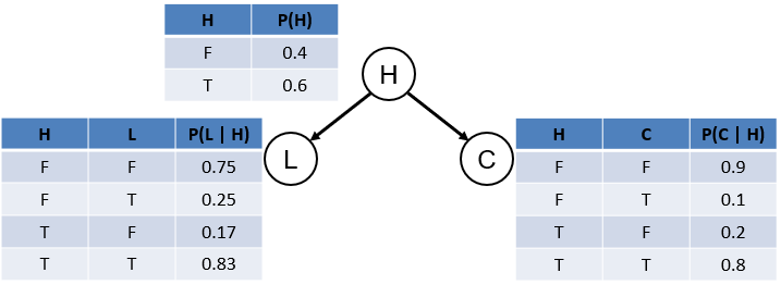
Recall our Solicitorbot Bayesian Network structure in which \(L \indep C~|~H\):
Alrighty -- let's take all of our probabilistic reasoning tools and put them together:
Firstly, we'll use our rearranging of the conditioning rule to re-write the joint: $$P(L, C, H) = P(L~|~C, H) P(C, H)$$ Why stop there?! We can factor again using the same rule, but this time on the \(P(C, H)\) term. $$P(L, C, H) = P(L~|~C, H) P(C~|~H) P(H)$$ Almost done: let's zero in on the \(P(L~|~C, H)\) term; can we reduce this by knowing that \(L \indep C~|~H\)? You betcha! $$P(L, C, H) = P(L~|~H) P(C~|~H) P(H)$$
In terms of the BN structure, what is particular about the factorization: \(P(L~|~H) P(C~|~H) P(H)\)
It consists of factors that are of the format: \(P(\text{child}~|~\text{parents}) = P(\text{effects}~|~\text{causes})\)
This is the intuition behind the semantics of a Bayesian Network! We can factor the joint as a product of effects given their causes.
Bayesian Networks exhibit the Markovian Assumption (named after Russian mathematician Andrey Markov) stating that "All variables are independent of their non-descendants when given their parents."
In other words, once we know a variable's causes, information from non-descendant variables is irrelevant, since they tell us nothing more than knowing what the direct causes already tell us.
Consequently, the Markovian Factorization of the joint distribution is: \begin{eqnarray} P(V_1, V_2, V_3, ...) &=& \prod_{V_i \in \textbf{V}} P(V_i~|~parents(V_i)) \\ &=& \{\text{Product of all CPTs in the BN}\} \end{eqnarray}
With the Markovian Factorization, this gives us a clear definition for the semantics of a Bayesian Network:
Bayesian Networks parsimoniously represent the joint distribution by maintaining a conditional probability table for each "family" of variables, such that for any variable \(V_i\) we know: \(P(V_i~|~parents(V_i))\)
In our example, this would look like the following:
"But hark!" you remark. The joint distribution had 8 rows to remember, but here we have 10 -- what gives? Wasn't the whole point to reduce the amount of probabilities we needed to store?
Observe the following highlights in the conditional probability tables and consider how we might be able to reduce the number of rows in our CPTs that we must remember:
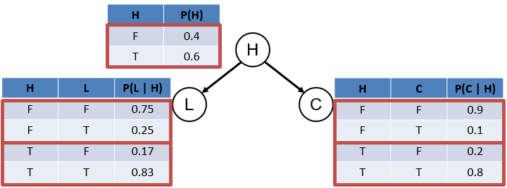
They all need to sum to 1! As such, we need only store 1/2 of these rows since their complements can be inferred via: \(P(\lnot \alpha) = 1 - P(\alpha)\)
Note: in general, we only need \(|V|-1\) values where \(|V|\) is the number of values in a variable. Above, we reduce by 1/2 because \(|V| = 2\) for binary variables.
As such, we now have:
Note: we now have parsimoniously represented the joint (8 rows) with factored CPTs (5 rows).
This might seem like a trivial savings, but we have a very small network with 3 variables that we have already been able to significantly shrink -- think of the savings at scale!
From the CPTs alone, we can make some simple inference queries, though more complex inference queries require inference algorithms that we will discuss next lecture.
Here are some inference queries we can compute from the above:
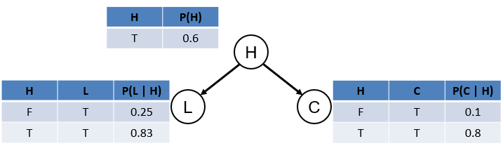
What is \(P(H = false)\)?
Using the CPT on \(H\), we see that \(P(H = false) = 1 - P(H = true) = 0.4\)
Indeed, if we want, we can simply reconstruct any row of the joint distribution by using the Markovian factorization and then multiplying consistent rows of CPTs:
What is \(P(H = false, L = true, C = false)\)?
Using all of the CPTs, we simply multiply the row consistent with the query in each: $$\begin{eqnarray} P(H = false, L = true, C = false) &=& P(L = true~|~H = false) P(C = false~|~H = false) P(H = false)\\ &=& 0.25 * 0.9 * 0.4\\ &=& 0.09 \end{eqnarray}$$
And that's Bayesian Networks in a (well... pretty big) nutshell!
Next week, tune in for more complex inferences!