To motivate exact inference, let's start with some review of what we've learned of Bayesian Networks, and use that to catapult into some inference techniques using them.

Review and Motivation

---

Before we do anything, we should ask:

What does inference mean in the context of Bayesian Networks?

BN inference seeks to estimate some probabilistic query of the format: $$BN.ask(\text{Query}, \text{evidence}) = P(Q | e)$$

Why might answering probabilistic inference queries be important to an artificial agent?

An agent may possess uncertainty about its environment, but is still required to make the most educated guess about its state as possible; recall, for example, the Solicitorbot that only wants to visit homes in which residents are present (but the bot may not know for certain if someone is home, yet can improve the accuracy of its guess based on observed evidence).

As such, we can see how probabilistic inferences help our agent's reason in spite of uncertainty, so why is this not straightforward?

Query Difficulty

---

As such, we need a means of answering inference queries in terms of the BN's parameters (i.e., how its semantics are stored / parameterized) alone.

What defines the network's "parameters?"

To answer that, let's look at what queries can be answered immediately from a BN and which require some additional computation.

O(1) Answerable Queries

---

How does a Bayesian Network factor the joint distribution over the network's variables? What factorization technique does it employ?

The Markovian Factorization of the joint, i.e., the joint factored into individual conditional probabilities of \(P(\text{effect}~|~\text{causes})\): $$P(V_1, V_2, V_3, ...) = \prod_{V_i \in \textbf{V}} P(V_i~|~parents(V_i))$$

How are these factors stored in the Bayesian Network? What defines the network's parameters / semantics?

At each node \(V\) in the graph, the factors are stored in conditional probability tables, which define: $$P(V~|~\text{parents}(V))$$

Putting the above together, what would constitute an inference query that we could answer immediately without any maths?

Any query that could be phrased as one of the known CPT quantities!

We'll consider an Immediately Answerable O(1) Query one that can be answered in \(O(1)\) directly from one of the network's CPTs / parameters (without needing to perform any computation).

Consider that these are stored in a map with known keys that describe the parent-child relationships for the quick look-up.

From there, since each CPT is literally a table, we should have O(1) lookup internal to these for given values of parents and child.

\(O(|V|)\) Answerable Queries

---

Of course, many of the queries we ask of our BN require some extra elbow-grease to answer. Here's the next simplest using a tool that we already know.

Linearly Answerable \(O(|V|)\) Queries (for \(|V|\) variables) are those that exploit the Markovian Factorization, since this is defined as a simple product over each variable's CPT: $$P(V_1, V_2, V_3, ...) = \prod_{V_i \in \textbf{V}} P(V_i~|~parents(V_i))$$

As such, any query which is simply a row of the joint distribution can be reconstructed by a product of CPTs in time linear to the number of variables.

How about one other tool from our past to help make some queries a little easier than the gory general case?

\(O(|V|^2)\) Answerable Queries

---

How do you think knowing the rules of d-separation, and the ability to perform it in \(O(|V|)\) can help answering some queries?

We can perhaps reduce some queries to those that *are* immediately answerable!

Quadratic Answerable \(O(|V|^2)\) Queries are those for which application of d-separation, with cost \(O(|V|)\), need be applied at most \(|V|\) times to reduce a query to a \(O(1)\) format.

This means that, perhaps we have some query with extra evidence that can be reduced to a format of a CPT, we can simply invest a little extra effort (which will usually be closer to \(O(|V|)\) for less evidence) to get to an easy query to answer.

For the following, simple Bayesian Network, determine which of the queries that follow are answerable in \(O(1), O(|V|), O(|V|^2)\), or none of the above; unless "none of the above", describe the steps needed to answer them.

Note: for brevity, I (and other representations) will sometimes use (0, 1) in place of (false, true) for Boolean variables, as is done in our Medibot diagnostic robot example below.

$$P(B = 0 | A = 1)$$

\(O(1)\) from the CPT on \(B\): $$P(B = 0 | A = 1) = 0.1$$

$$P(C = 1 | A = 1, B = 0)$$

\(O(|V|^2)\), since this can be reduced to an IA query by exploiting the independence claims of the network: $$\(C \indep A~|~B\)~\therefore~P(C = 1 | A = 1, B = 0) = P(C = 1 | B = 0)$$

$$P(A = 1 | B = 0)$$

None of the above -- there is no CPT with this quantity, and A is not d-separated from B, and so it must be computed.

$$P(A = 1, B = 0, C = 0)$$

\(O(|V|)\) since this can be computed from the Markovian factorization using all \(|V|\) factors in the network.

In recap, knowing the network's independence claims can reveal immediately answerable queries that may appear to be a required computation...

...but this comes at the cost of performing linear d-separation!

So, reasonably, one might observe that there are other queries that are interesting but not immediately answerable, nor linearly so -- how do we compute those?

Computable Queries

Computable queries, by contrast, are those that can be computed from a BN's parameters using the rules of probability theory. All queries are computable, but only some (detailed above) can be obtained efficiently.

Thus, we'll assume that the tools discussed herein pertain to when a query cannot be answered either instantly or linearly as described above.

The trick of computing any arbitrary BN query is to the use the information from the joint distribution over the network's variables without needing to fully reconstruct the joint distribution.

In addition to the Markovian Factorization of a Bayesian Network, the tools we'll need to remember to accomplish this are:

So how do we put it all together?

Enumeration Inference is an inference algorithm that can compute any query via sums-of-products of conditional probabilities from the CPTs.

Enumeration Inference works by selectively reconstructing parts of the joint needed to answer a query as a function of only the CPTs alone.

Disclaimer: Enumeration Inference, although the easiest to perform by-hand, is a brute-force approach that suffers exponential performance issues.

More sophisticated inference algorithms have addressed some of these computational problems (see a dynamic programming approach called Variable Elimination), but probabilistic inference is not an easy problem.

Variable Elimination and other advanced techniques can be covered in full graduate courses on their design, and are, unfortunately, out of scope for this class.

The Enumeration-ASK algorithm in Figure 14.9 of your textbook details a procedure for accomplishing this exact inference approach, but we'll examine the steps for performing it by hand below.

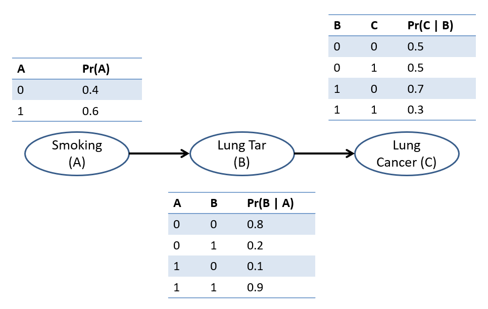
Motivating Example

Returning to our Medibot diagnostic system, let's answer a very important query: what is the likelihood of attaining lung cancer given that you smoke? $$P(C~|~A = 1) = ???$$

Step 1: Identify Variable Types

Enumeration inference begins by categorizing BN variables as one of three types for a query \(P(Q~|~e)\):

• Query Variable \((Q)\), is a single variable for which we are interested in computing the likelihood (more sophisticated inference algorithms can compute joints of query variables, but we'll keep it simple to start).

• Evidence Variables \((e)\), are variables that are observed at some value, and are held as evidence (note: lower-case \(e\) because these variables are fixed to their observed value \(E = e\)).

• Hidden Variables \((Y)\), are any variables in the network that are not part of the query (i.e., are neither query nor evidence variables).

In our Medibot example, what are the query, evidence, and hidden variables?

Query = \(\{C\}\), Evidence = \(\{S = 1\}\), Hidden = \(\{B\}\)

Intuitively, we want to compute the effect that Smoking (A) has on Lung Tar (B) deposits, and thus, the resulting effect that Lung Tar has on Cancer (C).

However, because Lung Tar is not a part of our query, it serves only as an "open valve" of information through which info about C flows from A.

Recap: we want to compute \(P(Q | e)\) but we only have the Markovian Factorization of the joint: \(P(Q, e, Y)\). So, we need to find a way to express what we *want* in terms of what we *have*.

Roadmap: To phrase our query \(P(Q | e)\) in terms of our MF, we have: $$\begin{eqnarray} P(Q~|~e) &=& \frac{P(Q, e)}{P(e)}~ \text{(Conditioning)} \\ &=& \frac{1}{P(e)} * P(Q, e)~ \text{(Algebra)} \\ &=& \frac{1}{P(e)} * \sum_{y \in Y} P(Q, e, y)~ \text{(Law of Total Prob.)} \\ \end{eqnarray}$$ Observe that \(P(Q, e, y)\) is the joint distribution, which we know how to factor using the Markovian Factorization!

Since we don't want to compute \(P(e)\) separately, as its own inference query, we'll exploit the fact that we can use the law of total probability on the intermediary computation of \(P(Q, e)\) to get it for free along the way!

Step 2.1: Compute \(P(Q, e) = \sum_{y \in Y} P(Q, e, y)\)

From our roadmap above, Step 2 is to phrase our query as a summation over the full joint via the network's markovian factorization, and worry about normalizing by \(P(e)\) at the end.

In other words, let's focus on finding: \(\sum_{y \in Y} P(Q, e, y)\).

For our Medibot example above, how would we write \(\sum_{y \in Y} P(Q, e, y)\) (the "template") for our variables found in Step 1? How to decompose the joint using the Markovian Factorization?

$$\sum_{y \in Y} P(Q, e, y) = \sum_{b \in B} P(C, A = 1, B = b) = \sum_{b \in B} P(C|B = b) P(B = b|A = 1) P(A = 1)$$

[Optional] Step 2.2: Optimizing Order

Notice that, above, our summation is somewhat naively constructed.

In the summation above (repeated below), knowing that every variable is binary, how many expressions will be summed? How many factors are in each summed expression? $$\sum_{b \in B} P(C|B = b) P(B = b|A = 1) P(A = 1)$$

We have two summed expressions consisting of 3 factors each, for a total of 6 factors that need to be evaluated (for a single value of \(C\)): $$P(C|B = 0) P(B = 0|A = 1) P(A = 1) + P(C|B = 1) P(B = 1|A = 1) P(A = 1)$$

Reasonably, we might consider whether every factor need be included in every summed term, or if we can save some computational effort by extracting terms that do *not* rely on the summation.

Looking back at the original summation, are there any factors that are unnecessarily repeated in the summation, and can be pulled outside?

Yes, the \(P(A = 1)\) factor can be pulled outside (since it has the same value in each iteration of the summation), thus reducing the number of evaluations required, and improving computational efficiency.

This gives us a new, equivalent expression that is more parsimonious! $$\sum_{b \in B} P(C|B = b) P(B = b|A = 1) P(A = 1) = P(A = 1) \sum_{b \in B} P(C|B = b) P(B = b|A = 1)$$

Notice that in this new expression, we have only 5 total factors to evaluate: $$P(A = 1) \sum_{b \in B} P(C|B = b) P(B = b|A = 1) = P(A = 1) [P(C|B = 0) P(B = 0|A = 1) + P(C|B = 1) P(B = 1|A = 1)]$$

This optimization (nontrivial for large networks) is implemented in the Enumeration-ASK algorithm by constructing an expression tree and using DFS, and can take a sum-of-products over \(|V|\) binary variables from a computational complexity of \(O(|V|*2^|V|)\) and reduce it to \(O(2^|V|)\).

Plainly, this is still a non-trivial computational cost, which is improved upon by more modern algorithms like Variable Elimination, which we will not have time to cover in here.

Rule of Thumb: to accomplish Step 2.2 by hand, it is easiest to arrange Markovian Factors in "topological order" (i.e., parents first and children second), then see if each factor, in sequence, can be moved outside of the summations.

Step 2.3: Do the damn thing

At this point, we have an expression that is ready to be computed using the network's parameters, so it's time to execute it!

Notice that our factors have been carrying the variable \(C\), indicating that we must compute the expression for each value of \(C\), giving us:

\(C\)	\(P(C,A=1)\)
\(C = 0\)	$$\begin{eqnarray} P(C=0,A=1) &=& P(A = 1) \sum_{b \in B} P(C = 0|B = b) P(B = b|A = 1) \\ &=& P(A = 1) [P(C = 0|B = 0) P(B = 0|A = 1) + P(C = 0|B = 1) P(B = 1|A = 1)] \\ &=& 0.6 * [0.5 * 0.1 + 0.7 * 0.9] \\ &=& 0.408 \end{eqnarray}$$
\(C = 1\)	$$\begin{eqnarray} P(C=1,A=1) &=& P(A = 1) \sum_{b \in B} P(C = 1|B = b) P(B = b|A = 1) \\ &=& P(A = 1) [P(C = 1|B = 0) P(B = 0|A = 1) + P(C = 1|B = 1) P(B = 1|A = 1)] \\ &=& 0.6 * [0.5 * 0.1 + 0.3 * 0.9] \\ &=& 0.192 \end{eqnarray}$$

Observant readers will note: "Hey! That doesn't sum to 1!" Well, luckily, we have our final step remaining...

Step 3: Find \(P(e) = \sum_{q \in Q} P(Q, e)\)

Recall our original roadmap, which was to compute: $$P(C~|~A = 1) = \frac{1}{P(A=1)} \sum_{b \in B} P(C, B = b, A=1)$$

What we just did was to compute \(\sum_{b \in B} P(C, B = b, A=1)\) but, this isn't our final answer!

The key, missing component, as you see, is our normalizing constant, \(\alpha = \frac{1}{P(A = 1)}\) (divides by the probability of the evidence).

Now, it just so happens that we have \(P(A)\) in the CPT of \(A\), but if we didn't happen to have evidence that was an immediately answerable query, what do we do?

Well, take another look at what we computed in the previous step, and observe what we actually computed: $$P(A = 1) \sum_{b \in B} P(C|B = b) P(B = b|A = 1) = P(C, A=1)$$

So, to find \(P(A = 1)\), all we have to do is sum up the remaining probability mass: $$P(A=1) = \sum_{c \in C} P(C = c, A=1) = P(C = 0, A=1) + P(C = 1, A=1) = 0.408 + 0.192 = 0.600$$

We can quickly verify that this is indeed the correct measurement for \(P(A = 1)\) from the CPT on \(A\)!

As such, we have that: $$\alpha = \frac{1}{P(A = 1)} = \frac{1}{0.6}$$

Step 4: Normalize \(P(Q | e) = \frac{P(Q, e)}{P(e)}\)

We'll take our joing marginal from step 2 \(P(Q, e)\), and our normalization factor from step 3 \(P(e)\) we now have our final answer to the query:

\(C\)	\(P(C~|~A = 1)\)
\(C = 0\)	$$\begin{eqnarray} P(C = 0~|~A = 1) &=& \frac{1}{P(A=1)} \sum_{b \in B} P(C = 0, B = b, A=1) \\ &=& \frac{1}{0.6} 0.408 \\ &=& 0.68 \end{eqnarray}$$
\(C = 1\)	$$\begin{eqnarray} P(C = 1~|~A = 1) &=& \frac{1}{P(A=1)} \sum_{b \in B} P(C = 1, B = b, A=1) \\ &=& \frac{1}{0.6} 0.192 \\ &=& 0.32 \end{eqnarray}$$

And there you have it! Our final answer: apparently smokers have a \(32\%\) chance of attaining lung cancer according to my fake data!

How about a little inference practice with our old friend the Solicitorbot (closure from some of our unanswered queries, and what not).

Don't worry yourself over small details like the table design and colors being different between this BN and the one above, variety is the spice of life.

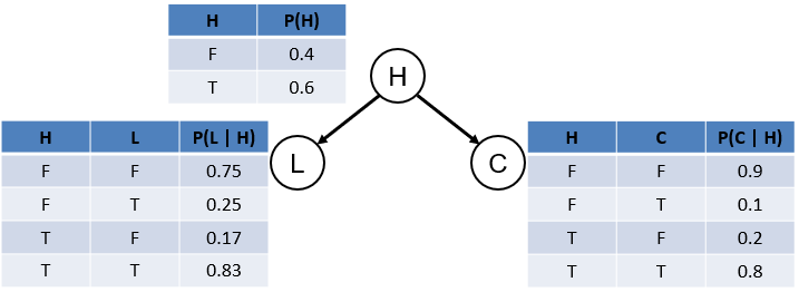
Determine the probability that a cacophony is heard in the house if a house's lights are on (click for solution and steps). $$P(C~|~L = 1) = ???$$

Determine the probability that someone is home given that a cacophony is heard inside and the lights are on (click for solution and steps). $$P(H~|~L = 1, C = 1) = ???$$

WHEW! That's a lot of maths! Once again teaching us an important lesson: this is why we have computers.

Given how hard enumeration inference is, we should look at some important efficiency improvements that get rolled into the Factor Elimination algorithm that we hinted at above.

Though we don't have time to look into factor elimination in detail, we can still learn from its tricks at a high level:

Efficiency Improvements

---

As our motivating example, we'll use your textbook's BN relating to some wonky alarm system [A] that goes off when either an Earthquake [E] or Burglary [B] triggers it, which then triggers nosy neighbors John [J] and Mary [M] to call you to let you know your alarm's going off.

Yes, this example is in the most used AI textbook to date.

In any event, it looks like the following:

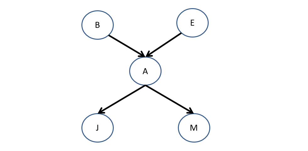
Now, suppose we wanted to compute the following queries (we'll ignore the normalizing constant for now just representing it as \(\alpha = \frac{1}{P(A=a, E=e)}\)):

Example 1: \(P(B | A = a, E = e)\) (i.e., find the likelihood of getting BAE)

\begin{eqnarray} P(B | A = a, E = e) &=& \alpha~\sum_j \sum_m P(B) P(E = e) P(A = a | B, E = e) P(J = j | A = a) P(M = m | A = a) \\ &=& \alpha~P(B) P(E = e) P(A = a | B, E = e) \sum_j P(J = j | A = a) \sum_m P(M = m | A = a) \end{eqnarray}

What do we notice about an interesting simplifying opportunity in the above equation?

The final two summations, i.e., \(\sum_j P(J = j | A = a)\) and \(\sum_m P(M = m | A = a)\) both sum to 1 by definition!

It turns out that this isn't a quirk, and allows for a general rule:

As such, we can simplify to:

$$P(B | A = a, E = e) = \alpha~P(B) P(E = e) P(A = a | B, E = e)$$

Simplification 1: Any hidden variable that is not an ancestor of a query or evidence variable is irrelevant to the query, and can be removed before evaluation.

Convenient, and intuitive! We'll end up summing over all of their values anyways, thus vacuously summing to 1.

Let's try another...

Example 2: \(P(B | J = j, M = m)\)

Here, we don't get to use our simplification #1 since all of the hidden variables are ancestors of the evidence, and therefore relevant.

However, there's a new concern to quell. Let's again write out our query roadmap:

\begin{eqnarray} P(B | J = j, M = m) &=& \alpha~P(B)\sum_e P(E=e) \sum_a P(A=a|B, E=e) P(J=j|A=a) P(M=m|A=a) \end{eqnarray}

Do we notice any potential inefficiencies that might be present in computing the equation above?

Yes! Note that in the second summation \(\sum_a ... P(J=j|A=a) P(M=m|A=a)\) will be repeated for multiple values of E in the outer sum: \(\sum_e ...\).

Note that this repetition can be order-dependent, so the order in which we choose to sum over hidden variables can have a serious impact on the amount of work that could be repeated.

So, let's not repeat ourselves!

Simplification 2: Never recompute a previously computed product of CPTs through clever use of memoization and dynamic programming.

The mechanics of doing *all of the above* are a little complex but exist in the context of an algorithm known as variable elimination.

We won't examine Variable Elimination in this class, but I highly encourage you to read through:

• Chapter 14.4.2 in your Textbook

• Related: The Jointree Algorithm mentioned in 14.4.4 of your Textbook.

Qualifying BN Inference Difficulty

---

It turns out that BN inference using Variable Elimination is easier in some cases than in others, and the computational difficulty will correspond to certain BN features.

What parts of a BN might affect inference difficulty, and what qualities of those parts would be computationally desirable?

The structure of a BN is closely tied to inference difficulty, with those that are tree-like in nature (see what I did there?) being more desirable.

In what other algorithmic paradigm did we see tree-structured-ness being a nice computational property?

The constraint graphs in Constraint Satisfaction Problems! It's all connected!

It turns out that tree-like structures lend themselves to easier application of the two simplifications mentioned above, and are easily exploited by Variable Elimination such that:

Networks that have a polytree / singly connected structure, i.e., for whom there is at most one undirected path between any node in the network, have complexity that is linear in the size of the network (i.e., size of CPTs).

Moreover, if there is an upper bound to the number of parents any node may have (common practice is to limit the in-degree at each node), computation will be linear in the number of nodes in the network as well.

The reasons for this benefit will be a bit handwavy (better explained by looking at those chapters above), but amounts to Variable Elimination having an easier time marginalizing / summing out variables in tree-like structures.

However, for non-polytree or multiply-connected structures, inference can be exponential in time and space and is an NP-Hard problem.

Draw some multiply-connected BN structures and consider why they will be more difficult.

For these reasons... maybe we can think about alternative strategies for inference different than exact computation...