Utility Theory
So we've seen some probability theory, we've seen some Bayesian stuff, we've more or less hinted at how probabilistic queries can be useful for intelligent agents, but importantly: we've only see hand-crafted examples wherein we (the humans) are making the queries!
Today's Teaser: how could an AI system translate their priorities and probabilistic understanding of a system into decisions?
Automating Priority
Our first task: how do we imbue agents with the notion of having different priorities, i.e., outcomes they wish to accomplish or avoid.
Consider some way for an agent to decide how desirable a given state (i.e., values of variables) is (Hint: some inspiration may be gleaned from adversarial search from Algorithms).
Some Utility Function / Score that assigned a numerical value to how good a state is -- the higher the better, baby!
We can use this formalization to guide an agent's actions even under uncertain conditions; as a reminder:
A Utility Function, \(U(s, a) = u\), maps some state \(s\) and action \(a\) to some numerical score \(u\) encoding its desirability.
Give some examples of some life events that may be subject to uncertainty but have different desirability of outcomes.
Some examples might include:
Applying to schools: getting into an Ivy League is great! ...but the probability is less than admittance into a state school and each application costs money.
Route planning: taking the freeway can be fast! ...but what if it's the 405 during rush hour / construction / accidents?
Playing the lottery: winning can be life-changing! ...but the probability is really low, and tickets cost money.
Consider the possible outcomes of a Utility function's outcomes for the state of winning a $1,000,001 lottery (s) and buying a $1 lotto ticket (a):
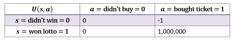
Namely:
\(U(s,a) = 10,000,000\) for \(s =\) winning a $10,000,001 lottery (and \(a=\) buying a $1 ticket).
\(U(s,a) = -1\) for \(s =\) losing, having \(a=\) bought a $1 ticket.
\(U(s,a) = 0\) for not having bought a ticket (though in principle, you may even have some FOMO penalty like -0.1 for when \(U(s=1, a=0)\) if the lotto is won using your usual lucky numbers).
Utility scores can be either hand-coded in a top-down fashion, or learned in a bottom-up.
However, unlike in adversarial search wherein our agent's actions transformed the state in a certain fashion, sometimes we need to make the best decision we can under circumstances that are not completely under our control.
Winning the lottery is great! ...but it's extremely rare.
Decision-making under uncertainty crops up in a myriad of AI applications:
In Blackjack, sometimes the best move is to hit even when we have a 15, even though sometimes we will bust.
In Hearthstone, sometimes the best move is to play a card that relies on some random number generator, even though sometimes it will backfire.
In Online Advertising, we must choose the ad that most likely fits a user's profile, even though clickthroughs are somewhat rare.
As such, we need a formalization that marries the likelihood of some events happening with the desirability of those events.
Utility Theory
Utility theory comes in handy when our agent must still attempt to act optimally even when its actions may have uncertain outcomes.
We should be wary to weight the really good outcomes proportional to their likelihood of happening, and perhaps instead settle for a lesser good that is more likely to happen.
Given the development of some Utility Function, and the notion of each state having some *chance* of occurring, can we devise some means of combining the two for informing a deciding agent?
We should be able to come up with a weighted utility score where the utility of each state is weighted by its likelihood of occurring!
These considerations are filed under the heading of *expected* utility:
The Expected Utility (EU) of some action \(a\) given any evidence \(e\) is the average utility value of the possible outcome states \(s \in S\) weighted by the probability that each outcome occurs, or formally: $$EU(a | e) = \sum_{s \in S} P(s | a, e) * U(s, a)$$
Note: \(P(s | a, e)\) in the above formula would be some sort of probabilistic query we would need the tools of past lectures to compute!
Rooted back to our Lottery example above, let's compute the EU of each action assuming:
There's no evidence, so \(e = \{\}\)
Whether or not we buy a lotto ticket has no affect on chances of winning, viz., \(S \indep A\):
The odds of winning the lotto are \(P(S=1) = 0.0000001\)
\begin{eqnarray} EU(A=1) &=& \sum_s P(S=s|A=1) * U(S=s, A=1) ~~~\text{(BUT since S and A are independent...)} \\ &=& \sum_s P(S=s) * U(S=s, A=1) \\ &=& P(S=0) * U(S=0, A=1) + P(S=1) * U(S=1, A=1) \\ &=& 0.9999999 * -1 + 0.0000001 * 1,000,000 \\ &=& -0.8999999 \\ EU(A=0) &=& ... \text{repeating the above though noting it's all 0 utility} \\ &=& 0 \end{eqnarray}
So, using the above, which action should we choose if we're a rational agent?
Plainly, then, if we're considering between some number of actions \(a \in A\) with uncertain outcomes, which action should we choose?
The one that maximizes the expected utility, of course!
Wasn't it The Rolling Stones who said, "You can't always get what you want, but if you try sometimes you might find... maximizing your expected utility to be sufficient?"
The Maximum Expected Utility (MEU) criterion stipulates that an agent faced with \(a \in A\) actions with uncertain outcomes (and any observed evidence \(e\)) shall choose the action \(a^*\) that maximizes the Expected Utility, or formally: $$MEU(e) = max_{a \in A}~EU(a | e)$$ $$a^* = \argmax_{a \in A}~EU(a | e)$$
To understand the difference between max and argmax, consider their types declared as (for some abstract action object):
\(MEU(e) \rightarrow\)
float\(a^* \rightarrow\)
action
Back to the lottery example:
\begin{eqnarray} MEU(\emptyset) &=& max_a~EU(a) \\ &=& max(EU(A=0), EU(A=1)) \\ &=& max(0, -0.8999999) \\ &=& 0 \\ a^* &=& \argmax_{a}~EU(a) \\ &=& \argmax(EU(A=0), EU(A=1)) \\ &=& A=0~ \text{(i.e., choose A=0)} \end{eqnarray}
By extension, suppose we had an in with the Lottery Mafia who guaranteed us a winning ticket, i.e., we knew that \(e = {S = 1}\) -- how would that change the above?
Now, suddenly, that \(A = 1\) action is looking a lot better!
Also, if you know anyone in the Lottery Mafia, let me know.
Notice: the above relied on understanding the potentially intricate structure relating probabilities, actions, and utilities -- let's think of a way to structure what we did above for any arbitrary system!
Decision Networks
The simple example in the previous section gives us a taste for the value of utility theory, but plainly, whenever we see some expressions of probability in the mix, we know that's just the tip of what could be a very large iceberg.
Indeed, when utilities are based on nontrivial relationships of cause and effect between variables in the system (sometimes through relationships that our agent cannot control), our agent should have a means of modeling these relationships to best inform its decision-making.
Naturally, then, pairing Bayesian Networks with Utility Theory seems like a nice way to enable autonomous, probabilistic reasoning.
Basics
A decision network unifies the stochastic modelling capacities of a Bayesian network with action-choice and utility theory by adding two additional nodes to the Bayesian network model. In particular, decision networks specify:
Chance Nodes (Circles) are traditional Bayesian Network variable nodes encoding chance in CPTs.
Decision Nodes (Rectangles) represent choices that the agent has to make, and can be used to model influences on the system. In certain contexts, decision nodes are referred to as interventions.
Decision nodes behave as follows:
Decisions have no CPTs attached to them; all queries to a decision network are assumed to have each decision node as a "given" since we are considering the utilities of different decisions.
Though treated like evidence in other CPTs, we do not need to normalize by their likelihood.
In CMSI 4320, we'll see how decision nodes are more clearly defined as part of the \(\mathcal{L}_2\) of the causal hierarchy, which uses a different notation for them.
Utility Nodes (Diamonds) encode utility functions, wherein parents \(pa\) of utility nodes are the arguments to the utility function, \(U(pa)\). Parents of utility nodes can be chance nodes OR decision nodes!
As a result, we can ammend the format of our EU computation in terms of decision network nodes: $$EU(a | e) = \sum_s P(s | a, e) * U(pa)$$
\(a\) is the action / decision being evaluated
\(s\) represents the "state nodes" or *chance node parents* of the utility node (the chance variables we care about scoring)
\(e\) is any known evidence about a chance node
\(pa\) are the parents of the utility node, which may be any combination of action and state based on the network structure.
Decision networks are useful for modeling complex probabilistic relationships between variables in the system while still attempting to maximize the utility of some decision that need be made.
Note that the CPTs of chance nodes will treat decision nodes as parents like any other cause-effect relationship in a Bayesian Network, even though decision nodes have no attached CPT since they are intentional actions being chosen with some certainty by the agent.
Hows about an example?
Example
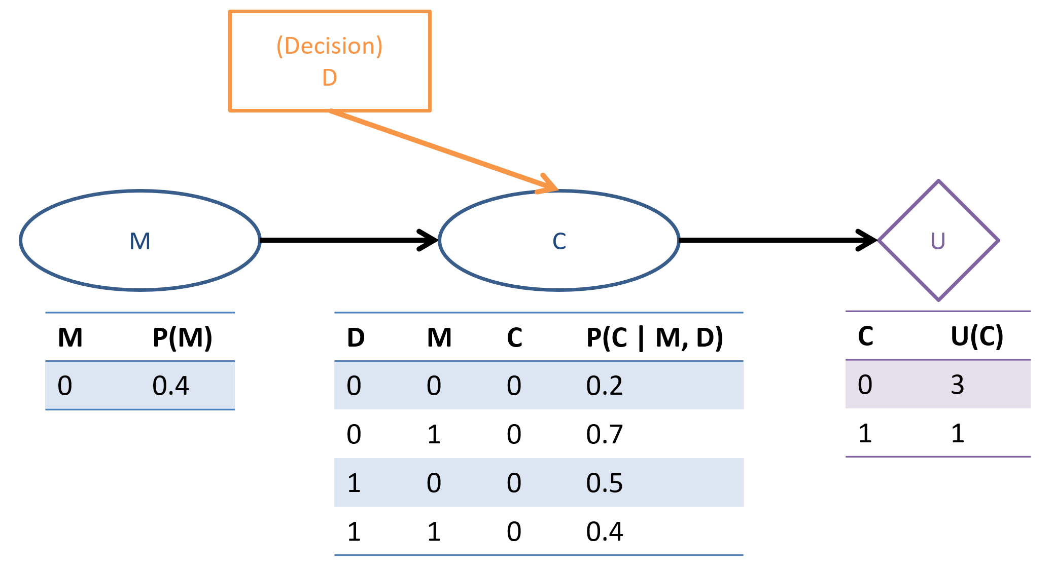
UX Designer: You're designing the interface for a banking app that customizes its appearance based on user demographics:
Chance nodes:
User Maturity \(M \in \{\text{young}, \text{old}\} = \{0, 1\} \): important for tailoring interface elements towards investment strategies.
User Complaints \(C \in \{0, 1\}\): feedback gathered about site experience.
UX Decision \(D \in \{0, 1\}\): whether to highlight interface elements for retirement savings or investments.
Utility Node \(U(pa) = U(C)\): score of whether or not users complain (note: decision D only affects the utility through C).
Using the MEU criteria, and the Decision Network specified above, which interface display decision \(D = \{0, 1\}\) should our app make when the user's age is not known (i.e., when \(M\) is hidden)?
We'll have to compute the EU of each decision, and then choose the best, of course!
This procedure will look a lot like Enumeration Inference, but with some key differences.
Roadmap: to remind ourselves of what we're trying to find, let's examine the EU definition: \begin{eqnarray} EU(a | e) &=& \sum_{s \in S} P(s | a, e) * U(pa) \\ &=& \sum_{\text{Chance node state s that are parents of U node}} \{\text{BN Query for likelihood of s | a, e}\} * \{\text{Utility of pa}\} \end{eqnarray}
Note the main differences from Enumeration Inference:
The decision variable \(D\) is treated like evidence, but requires no normalization for the likelihood of the evidence because it has no attached CPT.
Note that we also must sum over all values of the chance-node-parents of the utility node, which includes all *combinations* of parent values in the case of multiple chance-node parents.
Thus, if we find the distribution \(P(S | a,e)\) via our standard inference procedure, we can plug this into our EU computation for each value \(s \in S\).
Step 1: Compute \(P(S | A, e)\)
Note the capital \(S, A\) here, indicating that we want to find the *distribution* over S for ALL values of our decision / action \(A\) given evidence \(e\).
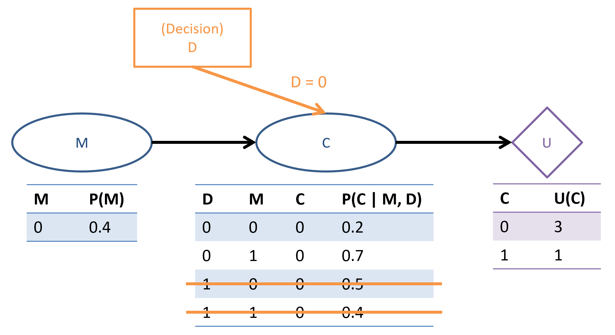
Let's start out with \(D = 0\), which thus configures our network into the world where \(D = 0\):
Step 1.1 - Label Variables: only difference here is that we need to add a new label for our decision variables, \(D\), which are treated slightly different than evidence.
\(Q=\{C\}, e=\{\}, D=\{D\}, Y=\{M\}\)
Step 1.2.1 - Find \(P(Q, e | D) = \sum_y P(Q, e, y | D)\): no that's not the end of a proof (QED joke?), but notice that the only difference here is that our decision variable is added to the mix, so with no evidence \(e = \{\}\) we get: \begin{eqnarray} P(Q, e | D) &=& P(C | D) \\ &=& \sum_m P(C, M = m | D) &\text{(Law of Total Prob.)}\\ &=& \sum_m P(C | M=m, D) P(M=m | D)~~~&\text{(Conditioning)} \\ &=& \sum_m P(C | M=m, D) P(M=m) &(M \indep D) \\ \end{eqnarray}
Note that the above is just the Markovian Factorization but with decision-node parents of chance nodes where appropriate in the model.
Step 1.2.2 - Optimize Summation Order: We would typically try to optimize order of summations like in Enumeration Inference, but we cannot do so here since each CPT is dependent on the summation over \(m \in M\).
Step 1.2.3 - Compute: Time to Plug-and-Chug!
\(P(C | D)\) |
\(C=0\) |
\(C=1\) |
|---|---|---|
\(D=0\) |
\begin{eqnarray} &\sum_m& P(C=0 | M=m, D=0) P(M=m) \\ &=& P(C=0 | M=0, D=0) P(M=0) \\ &+& P(C=0 | M=1, D=0) P(M=1) \\ &=& 0.2 * 0.4 + 0.7 * 0.6 \\ &=& 0.5 \end{eqnarray} |
\begin{eqnarray} &\sum_m& P(C=1 | M=m, D=0) P(M=m) \\ &=& P(C=1 | M=0, D=0) P(M=0) \\ &+& P(C=1 | M=1, D=0) P(M=1) \\ &=& 0.8 * 0.4 + 0.3 * 0.6 \\ &=& 0.5 \end{eqnarray} (alternately: \(1 - P(C=0|D=0)\)) |
\(D=1\) |
\begin{eqnarray} &\sum_m& P(C=0 | M=m, D=1) P(M=m) \\ &=& P(C=0 | M=0, D=1) P(M=0) \\ &+& P(C=0 | M=1, D=1) P(M=1) \\ &=& 0.5 * 0.4 + 0.4 * 0.6 \\ &=& 0.44 \end{eqnarray} |
\begin{eqnarray} &\sum_m& P(C=1 | M=m, D=1) P(M=m) \\ &=& P(C=1 | M=0, D=1) P(M=0) \\ &+& P(C=1 | M=1, D=1) P(M=1) \\ &=& 0.5 * 0.4 + 0.6 * 0.6 \\ &=& 0.56 \end{eqnarray} (alternately: \(1 - P(C=0|D=1)\)) |
Step 1.3 - Find \(P(e|D) = \sum_q P(e, Q=q | D)\)
Since \(e=\{\}\) in our example, no normalization to be done!
Step 1.4 - Find \(P(Q | e, D) = \frac{P(Q, e | D)}{P(e | D)}\)
Since \(P(Q | e, D) = P(C | D)\) in our example, we already found the answer in Step 1.2. In general, we would have to normalize by Step 3 here.
Whew! So to recap above:
We computed the likelihood of every state value that the Utility function takes as a parameter (i.e., any parent of it in the decision network) so that next we can weight the utility of each state outcome by its likelihood.
Normally, you'd have a computer do this for you, of course, but essentially the process is the same as enumeration inference but with the values of a decision node always given in the query, and not needing to normalize by its likelihood (since decision nodes have no likelihood).
Seem like this is a bit wonky? Don't worry, we'll look at a more sophisticated view of decisions and interventions in CMSI 4320.
Now, on to the finale...
Step 2 - Find \(EU(a | e) = \sum_s P(s | a, e) U(s, a)~\forall~a\)
For our example, since there is no evidence, this means that we must find \(EU(D)~\forall~d \in D\)
\begin{eqnarray} EU(D=0) &=& \sum_{c} P(C = c | D = 0) U(C = c, D = 0) \\ &=& P(C=0|D=0) U(C=0) + P(C=1|D=0) U(C=1) \\ &=& 0.5 * 3 + 0.5 * 1 \\ &=& 2 \\ EU(D=1) &=& \sum_{c} P(C = c | D = 1) U(C = c, D = 1) \\ &=& P(C=0|D=1) U(C=0) + P(C=1|D=1) U(C=1) \\ &=& 0.44 * 3 + 0.56 * 1 \\ &=& 1.88 \\ \end{eqnarray}Those were the hard parts! Finally, we just pick the best...
Step 3 - Find \(a^* = \argmax_{a \in A} EU(a | e)\)
Since \(EU(D=0) \gt EU(D=1)\), we have a winner!
Looks like \(D = 0\) is the way to go here!
Repeat the above under the assumption that we *know* the age of the user: \(M = 0\).