Value of Perfect Information

Today we look at a topic very closely related to Decision Networks and Utility Theory, and one that might feel vaguely related to a dilemma faced by an agent in a previous assignment...

In your BlindBot assignment, you may have taken moves that were not directly aimed at the goal, but instead at more safely navigating the environment and attempting to pinpoint previously ambiguous pit locations.

In taking these extra, exploratory moves, BlindBot still incurred some minor cost (that battery was draining quickly!), but that cost could be offset if the investment helped navigate around a pit!

This is true of many decision-making tasks: we're often willing to go a little bit out of our way to gather extra information if it means making a better decision overall.

In other words, we might say that extra information has some *value* in terms of our utility function that our agent is still attempting to maximize.

While some information may be worthwhile to take a detour to acquire, other info might not be, and we should equip our agent to answer the very important question:

"Is the juice worth the squeeze?"

The Value of Perfect Information (VPI) computes the expected increase in utility from acquiring new evidence.

We'll see why it's termed "Perfect" information in a moment, but for now, let's consider a motivating example (warning, I took a traditional example and spiced it up a little with some maximal cringe).

Music Festival Tickets

You are debating whether or not to buy tickets to the upcoming Fyre Music Festival, but tickets are expensive and you'll only really enjoy it if the line-up is lit (lyt?). Still, you get fear of missing out (FOMO) quite easily, and there would be near irreparable social cost if you didn't attend (until the next music festival, at least).
The problem: tickets are on presale and are going to sell out before the entire line-up is listed, but your favorite band has neither confirmed nor denied their spot on the bill.
Your friend's friend, Mike (who always just seems to be around social gatherings, but was never particularly invited), claims that he knows a member of your favorite band, and will tell you whether or not they'll be there (thus making the line-up lyt)... if you give him $5 (the scumbag). You're not sold on Mike's reputation and think there's a decent chance he's just bumming $5 for some White Claw.

Your Task: determine if it's worth it to give $5 to Mike.

Knowing what you know now, how might you go about answer this?

We'd need to define a couple of things:

The likelihood that Mike will give us an honest, accurate answer as to our favorite band's attendance, and what it tells us about the band's likelihood of being at the concert.
How much we value attending / not attending the festival in all possible outcomes, i.e., our favorite band attending / not attending.

Oh hey, let's use a decision-network to do those things.

Because computing VPI requires uniting probabilistic distributions and utility scores, it can be computed directly from a specified decision-network.

For our example, suppose we come up with the following:

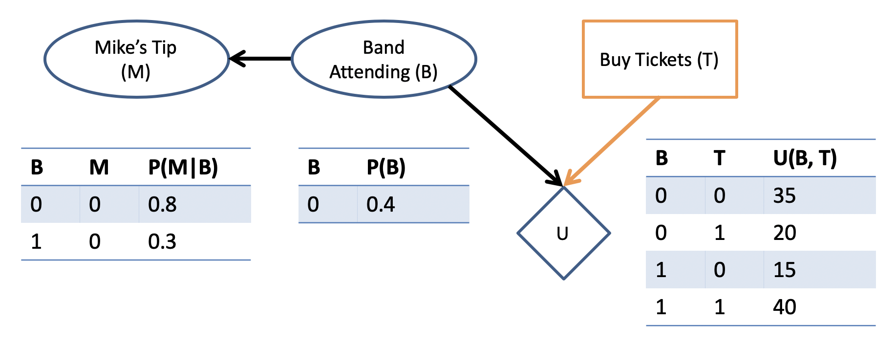
In general, these CPTs may come from data of past observations, and the utility may be based on some dollar-unit (e.g., "how much would you pay about a ticket cost to go see your favorite band?")

Just *how* we came up with those likelihoods and utility values in this example is a matter of debate (but if you were taking this example seriously, you're already doing it wrong).

Still, let's suppose those utility values are mappable to monetary amounts, and we can compare whether or not Mike's info is worth the cost.

Reflect: How do we go about that computing the value of Mike's information from the assumptions in our decision-network?

Defining VPI

The proceduralization of computing VPI stems from a couple of intuitive insights:

Insight 1: We will act optimally (i.e., according to the Maximum Expected Utility (MEU) criteria) with whatever information we have available to us, $(E = e)$.

Insight 2: We may act differently as soon as we acquire new information (about some other var $E'$).

How do we then combine these two insights to define VPI?

VPI = difference in maximum expected utility between having and not having the new information!

Formally, we can express that as:

Computing the VPI of observing some variable $E'$ for any *already* observed evidence $E = e$ is defined as the difference in maximum expected utility between knowing and not knowing the state of $E'$, written: $$VPI(E' | E = e) = MEU(E = e, E') - MEU(E = e)$$

In words, interpreting the above:

$VPI(E' | E = e)$ = The value of learning about the state of $E'$ if I already know $E = e$.
$MEU(E = e, E')$ = The maximum expected utility of me acting optimally knowing what I do now $E=e$, AND about the state of $E'$.
$MEU(E = e)$ = The maximum expected utility of me acting optimally knowing what I do now $E=e$.

This computation would be relatively straightforward were it not for a couple of snags:

We have to assess how each value of the evaluated variable $E'$ affects our decisions and the resulting utility (we might change our mind given some new evidence).
Since $E'$ is still a random variable, we need to weight our final assessment according to the likelihood of seeing each value of $E'=e'$ given our already observed evidence $E = e$.

Let's step back from words and definitions and depict what's going on.

We'll start by comparing the MEU of the case wherein we don't know anything about $E'$ and the case where we know it to be observed at some value.

Depicted below: a tree diagramming the MEU computation wherein triangles represent max-nodes (take the max value of their children), circles summation, and diamonds the utility map.

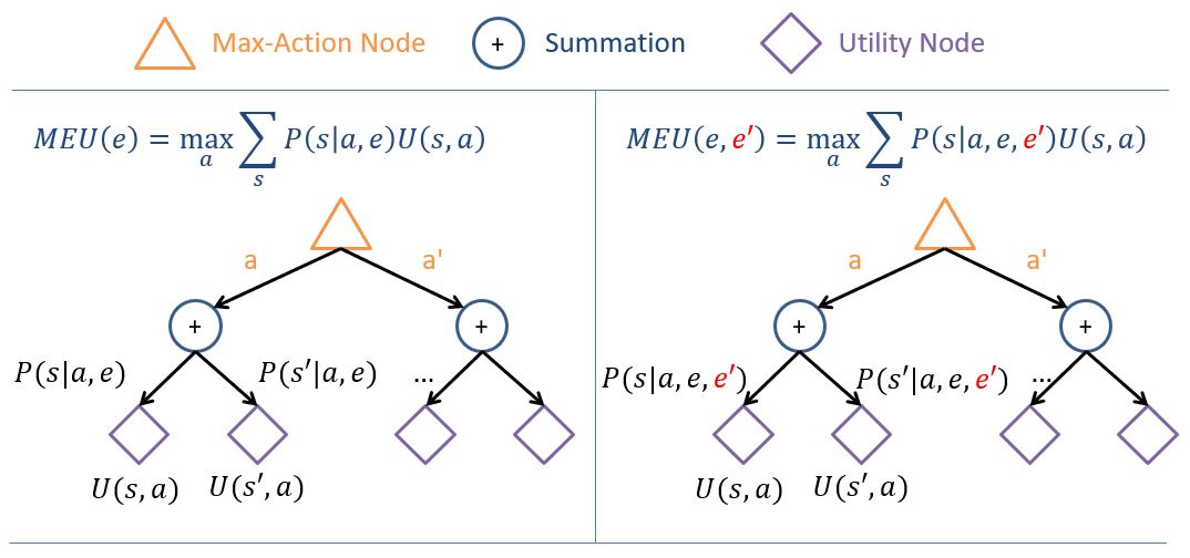
For our Music Festival example, the left represents our MEU if we didn't know anything going into it $E = \emptyset$ whereas the right would be our MEU if Mike gave us any one answer to whether or not our favorite band was going to play, $E' = e'$.

Note: the only difference is a change in the likelihood of being in each state.

However, this right tree is not the whole story, because as noted, when considering the VPI of $E'$, we have to think about its usefulness *contingent on the answer we get* for each of its states -- we don't know what answer we'll get in advance!

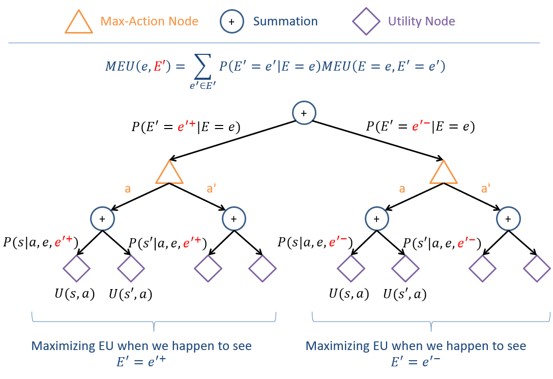
Each of these possible states $e' \in E'$ has some likelihood associated with it that must be updated by our observed evidence $E = e$, meaning we must assess:

The Maximum Expected Utility associated with the reveal of some variable $E'$ given some other evidence $E = e$ is the weighted sum over all values $e' \in E'$ of the likelihood of seeing $e'$ with the MEU of how we would act seeing $e'$, or formally: $$MEU(E = e, E') = \sum_{e' \in E'} P(E' = e' | E = e) MEU(E = e, E' = e')$$

Again, depicting this scenario, we see we have our right-most tree above but replicated and weighted by the likelihood of seeing each value $e' \in E'$:

Whew! What a tree. That tree makes you smile, sit back in your chair, smile ponderously, put your chin on your hand and think, "Damn... I'm educated."

Let's see how to actually do one of these examples by hand, hmm?

Proceduralizing VPI

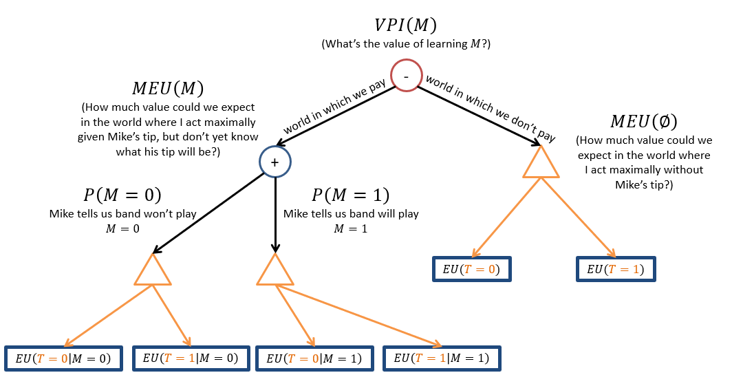
Returning to our Music Festival Example, let's go step by step computing $VPI(M)$ trying the reason over the above.

Remember that since we have no other information, $E=e$, we have: $$VPI(M) = MEU(M) - MEU(\emptyset)$$

Combining the tree-like depictions of our calculations above into plain-English descriptions, we have:

Step One: Find $MEU(E = e)$, i.e., MEU without knowing anything about $E'$.

In our example, this isn't too bad since $E = \emptyset$

For our problem, $MEU(E=e) = MEU(\emptyset)$ since there is no evidence. As such:

Step 1 - Find $P(S | A, e)$: For us, that's $P(S|A,e) = P(B | T) = P(B)$. Oh look! We already have that in the CPT.

Step 2 - Find $EU(a | e)~\forall~a$: that means:

\begin{eqnarray} EU(T = t) &=& \sum_s P(s|a, e) U(s, a) \\ &=& \sum_b P(B = b) U(B = b, T = t) \\ EU(T = 0) &=& P(B = 0) U(B = 0, T = 0) + P(B = 1) U(B = 1, T = 0) \\ &=& 0.4 * 35 + 0.6 * 15 = 23 \\ EU(T = 1) &=& P(B = 0) U(B = 0, T = 1) + P(B = 1) U(B = 1, T = 1) \\ &=& 0.4 * 20 + 0.6 * 40 = 32 \end{eqnarray}

Step 3 - Find $MEU(e) = max_a EU(a | e)$: Again, without evidence this gives us $MEU(e) = MEU(\emptyset) = 32$ based on the above.

Therefore, our $MEU(\emptyset) = 32,~\therefore~ a^* = \{T=1\}$, and it seems that buying a ticket for the show is the clear win.

Step Two: Find $MEU(E = e, E' = e')~\forall~e' \in E'$, i.e., the MEU of how we would act knowing each possible outcome of the variable being evaluated: $E'$.

In our Music Festival example, what is $E'$, and what values do we have to assess?

Our $E'$ is Mike's Tip $M$, and we must assess the MEU in each world where: (1) Mike tells us the band isn't playing, and (2) Mike tells us they are.

With that knowledge in tow:

Goal - Find $MEU(E = e, E' = e')~\forall~e' \in E'$: for us, without any added evidence $E=e$, that's $MEU(M)~\forall~m \in M$

Step 1 - Find $P(S | A, e)$: For us, that's $P(S|A,e) = P(B | M, T) = P(B | M)$, noting that our prospective variable $M$ is added as evidence.

Our first MEU computation was slightly easier because we have no additional information going into the problem, i.e., no $E = e$, but since Mike's Tip only tells us something about the utility through what it tells us about $B$, we'd need to compute $P(B | M)$ through standard inference. I've done that for us, to save some time:

Step 2 - Find $EU(a|e)~\forall~a$: Here, this is thus $EU(T | M)$. This means we'll need to compute this quantity for all combos of $T, M$.

\begin{eqnarray} EU(T | M = 0) &=& \sum_b P(B = b | M = 0) U(B = b, T = t) \\ EU(T=0 | M=0) &=& P(B = 0 | M = 0) U(B = 0, T = 0) + P(B = 1 | M = 0) U(B = 1, T = 0) \\ &=& 0.64 * 35 + 0.36 * 15 \approx 28 \\ EU(T=1 | M=0) &=& P(B = 0 | M = 0) U(B = 0, T = 1) + P(B = 1 | M = 0) U(B = 1, T = 1) \\ &=& 0.64 * 20 + 0.36 * 40 \approx 27 \\ \end{eqnarray}

Step 3 - Find $MEU(E=e, E'=e')$: $MEU(M=0) = max_t EU(T=t|M=0) = 28,~\therefore~ a^* = \{T=0\}$

Note: after observing $M=0$ above, we have a case where our decision would change to not buying the ticket, $T=0$!

I'll combine some steps for parsimony below, but note that we need to do the same thing as above for $EU(T | M=1)$.

\begin{eqnarray} EU(T | M = 1) &=& \sum_b P(B = b | M = 1) U(B = b, T = t) \\ EU(T=0 | M=1) &\Rightarrow& P(B = 0 | M = 1) U(B = 0, T = 0) + P(B = 1 | M = 1) U(B = 1, T = 0) = 13.2 \\ &=& 0.16 * 35 + 0.84 * 15 \approx 18 \\ EU(T=1 | M=1) &\Rightarrow& P(B = 0 | M = 1) U(B = 0, T = 1) + P(B = 1 | M = 1) U(B = 1, T = 1) = 45.2 \\ &=& 0.16 * 20 + 0.84 * 40 \approx 39 \\ &\therefore& MEU(M = 1) = 39 \end{eqnarray}

Whew! Alright, almost done...

Step 3: Find $MEU(E = e, E')$, the weighted sum of each individual $MEU(E = e, E' = e')$:

Again, this is easy because we have no observed $E = e$, but in general, would need to find $P(E' = e' | E = e)$.

I've done the easy job of simply finding $P(M)$, which, as it turns out, is $P(M = 0) = P(M = 1) = 0.5$ (totally planned, Mike that fickle f***).

\begin{eqnarray} MEU(E = e, E') &=& \sum_{e'} P(E' = e' | E = e) MEU(E = e, E' = e) \\ MEU(M) &=& \sum_{m} P(M = m) MEU(M = m) \\ &=& P(M = 0) MEU(M = 0) + P(M = 1) MEU(M = 1) \\ &=& 0.5 * 28 + 0.5 * 39 = 33.5 \end{eqnarray}

Step 4: Find $VPI(E' | E = e)$ by pluggin and chuggin.

\begin{eqnarray} VPI(E' | E = e) &=& MEU(E = e, E') - MEU(E = e) \\ &=& 33.5 - 32 = 1.5 \end{eqnarray}

Conclusions:

This is why we have computers.
Mike's dumb tip is only worth an expected utility increase of about 1.5; if we treat this as equivalent to dollar amounts, we would have to haggle him down to about a $1.50 to make his semi-trustworthy information useful.

VPI Properties

Now for the exciting part that everyone eagerly awaits: some properties of VPI!

First, motivated by a question that has also plagued philosophers for ages...

Is it ever possible for additional knowledge to be *harmful* to expected utility? i.e., could we have: $$MEU(E = e, E') \stackrel{?}{\lt} MEU(E = e)$$

Yes! Learning the value of some variable might make all of our decisions (under either of its values) look more grim than had we not known about it to begin with.

This would, however, make $VPI(E' | E = e) \lt 0$ -- why does this not make sense?

Information is only ever helpful (in that it helps to narrow down the possible state we're in), or useless, but never harmful, by definition, because we could always just ignore that information and be as well off as we were before seeing it.

Property 1: VPI is nonnegative such that: $$VPI(E' | E = e) \ge 0~\forall~E', e$$

Functionally, this means that any VPI computation whose difference between $MEU(E=e, E')$ and $MEU(E=e)$ is negative is simply capped at 0.

Knowledge is power!

This raises an interesting question, since we said it can be greater than *or equal to* 0.

Under what circumstances might $VPI(E' | E = e) = 0$?

When the evidence is irrelevant to the utility!

Generally, since a decision network still obeys the rules of d-separation, we can simply determine whether or not the variable being assessed tells us anything new about the utility node.

Property 2: The VPI of variables that are independent / conditionally independent from the utility node(s) will be 0, viz.: $$(E' \indep U | E = e) \Rightarrow VPI(E' | E = e) = 0$$

(where $(E' \indep U | E = e)$ is used to indicate that $dsep(E', U | E = e)$)

Suppose we added another variable related to Mike's Tip in our Music Festival Example, some variable $A$:

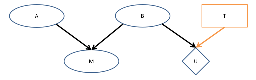
Are each of the following VPI queries zero or nonzero?

$VPI(A)$
$VPI(A | M)$
$VPI(A | M, B)$

Answers:

$VPI(A)$ = 0 since $A \indep U$
$VPI(A | M)$ = nonzero since $A \not \indep U | M$
$VPI(A | M, B)$ = 0 since $A \indep U | M, B$

Lastly, consider the fact that we might be interested in / offered the values of *two or more* variables like:

$$VPI(E'_i, E'_j | E = e)$$

This is indeed allowed, but we should be careful with how we compute the value of having multiple new pieces of evidence. To see where this danger comes from:

Is $VPI$ additive such that, for any arbitrary $E'_j, E'_k$: $$VPI(E'_j, E'_k | E = e) \stackrel{?}{=} VPI(E'_j | E = e) + VPI(E'_k | E = e)$$

No! This might give us overlapping value.

Consider having $VPI(M, B)$ in our previous example, in which $M$ provides no new value that $B$ doesn't already, but alone, each does have a positive VPI.

Property 3: VPI is non-additive such that: $$VPI(E'_j, E'_k | E = e) \ne VPI(E'_j | E = e) + VPI(E'_k | E = e)$$

(Note: although not true in general, this *might* be the case for some circumstances... can you think of what they are?)

However, not all hope is lost, since we can still compute the VPI on multiple query variables so long as we isolate the *portion* of utility that each query can provide information about.

Intuitively, this can be done by holding one of the two variables constant (i.e., as observed evidence) while computing the VPI of the other.

Property 4: VPI is order independent for computing the value of multiple queries so long as the others are held constant after their contribution to the utility has been evaluated (and the order doesn't matter): \begin{eqnarray} VPI(E'_j, E'_k | E = e) &=& VPI(E'_j | E = e) + VPI(E'_k | E'_j, E = e) \\ &=& VPI(E'_k | E = e) + VPI(E'_j | E'_k, E = e) \\ \end{eqnarray}

Think of this relationship as the "Conditioning" rule of VPI (it even looks a lot like it).

Whew! At this point you might be questioning the value of information in general -- too much can be enriching or crushing!

We'll chase this lecture with some practice next time around... see y'all at the Fyre Festival, I've heard good things from Mike.