Bayesian Networks: Approximate Inference
Thus far, we've seen techniques for computing solutions to exact queries in Bayesian Networks, including Enumeration Inference (in detail), Variable Elimination / Jointree (mentioned in the course notes / textbook).
In all cases, we might step back and ask some very reasonable questions about just how difficult inference is...
Insight 1: Since this is fuzzy logic, do we always care about getting precisely the right answer to our queries?
Not necessarily! Approximate solutions won't do us any favors for theorem proving, but they might get the job done for back-of-the-napkin computations.
Insight 2: Could we consider an alternative means of computing queries that might get us ballpark answers without as much of the computational strain?
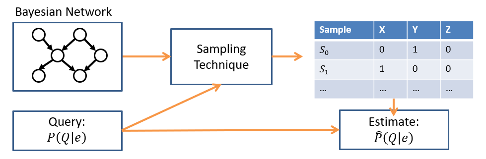
We could simulate / sample data consistent with the network CPTs, and use that data to answer queries of interest.
Sampling Basics
The process of sampling from some probability distribution is the ability to generate a "fake" data point that is consistent with the underlying distribution / training set / model.
We'll see sampling in a variety of contexts in this course, but let's establish some precedent for it with Bayesian Network inference first!
In the case of a Bayesian Network, since we are encoding the joint distribution through the network CPTs, we no longer have direct access to the JPT... but we *can* use the CPTs to generate samples from it.
Sampling is a common technique used in many computing sub-disciplines as a cost-effective means of generating good, but not perfectly accurate, answers.
Where else have you seen sampling techniques used? (Hint: think about to CMSI 186!)
To see why sampling is useful, let's consider a small (perhaps insultingly small, but meh), classic example:
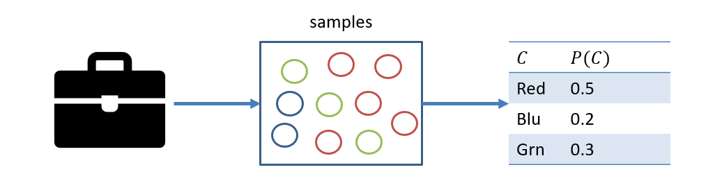
You have an attache case full of different-colored marbles and want to determine the relative distribution of any given color, with some caveats: (1) you cannot look into the bag to count them (there are too many), but (2) can remove one at a time and count it.
I wanted to make an example that was at least somewhat entertaining while remaining cliche; could you imagine a high-priced lawyer going to court with an attache full of marbles? The insanity defense would never look so good: "As you can see, your honor, my client has lost all of their marbles."
Anywho, let's think about this stupid scenario and use it as a springboard into more serious mechanics.
Q1: how would you go about establishing the distribution of colors in this case?
Continuously sample from it! (1) Pull a marble out at random, (2) record its color, (3) put back, repeat!
At the end of sampling many times, we get a reasonably accurate picture of the underlying distribution, depicted:
On what is the accuracy of our sample distribution reliant?
Primarily: Sample Size: we have to make sure we've sampled enough lest we suffer from sampling bias -- fewer samples means less accuracy.
By the same logic, if you flip a coin 10 times, and it comes up heads 8 / 10, you don't want to conclude that the chance of heads is 80%; you just flipped it too few times to get an accurate reading.
These ideas are summarized under a couple of formal ideas with which you should be familiar:
The Law of Large Numbers (briefly summarized) states that as the sample size trends towards infinity, the likelihood of some event converges to its true likelihood. Namely, for the number \(N_S\) of samples of some event \(N_{S}(x_1, x_2, ..., x_i)\) (with total number of samples \(N\)), we have:
$$lim_{N \rightarrow \infty} \frac{N_{S}(x_1, x_2, ..., x_i)}{N} = P(x_1, x_2, ..., x_i)$$A sampling strategy that guarantees the above result is said to be consistent.
Simulated Sampling
Of course, in the context of having probability distributions of a Bayesian Network, we don't have a physical case of marbles we draw from, so must instead simulate the sampling process through techniques broadly in the "Monte Carlo" paradigm.
Simply put, for us: we have some number of conditional probability tables from which we must generate fake data points that are consistent with that underlying distribution.
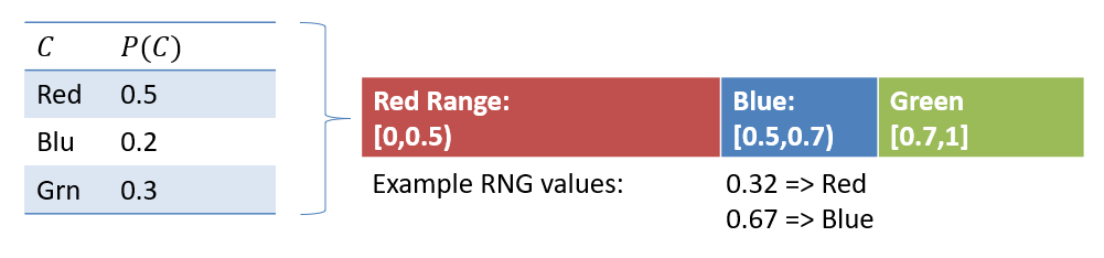
This can be accomplished quite simply through use of a random number generator and using the probability values in the table as a range through which to interpret the sample.
Consider the ability to use a number line partitioned on the various probability values of a distribution:
Importantly, from the above:
Note that the CHANCE that we sample each value from the distribution is proportionate to how likely it is in the table.
We can generate as many simulated data points from this as we please without having to worry about replacement.
You must be asking: if we have the distribution like \(P(C)\) above, why do we need to generate fake datapoints?
A: What if the distribution is a QUERY that you don't have immediately answerable? \(P(Q|e)\) Its answer will be distributed within the CPTs of a BN, but perhaps instead of performing a costly enumeration inference ask, we can instead sample to estimate its answer!
Sampling in a BN
Unlike in the previous example wherein we had a single variable (Color) and did not know the underlying distribution, sampling in a BN is a bit more complex for a couple of reasons.
Reflect: what are some challenges associated with sampling in Bayesian Networks?
There are multiple variables.
Some of those variables may be independent / conditionally independent.
We may want to assess samples on queries that are consistent with some evidence / observed value of certain variables.
However, with greater challenge comes greater expressiveness... let's start by considering the value / merit of sampling and how it applies to inference.
Answering Queries from Samples
Before we look at the means of sampling from a BN, let's consider the merit of doing so.
As is a tradition in all Bayesian Network classes, it's time for you to meet the most cliche of all reasoning systems: The Sprinkler Sidewalk Example.
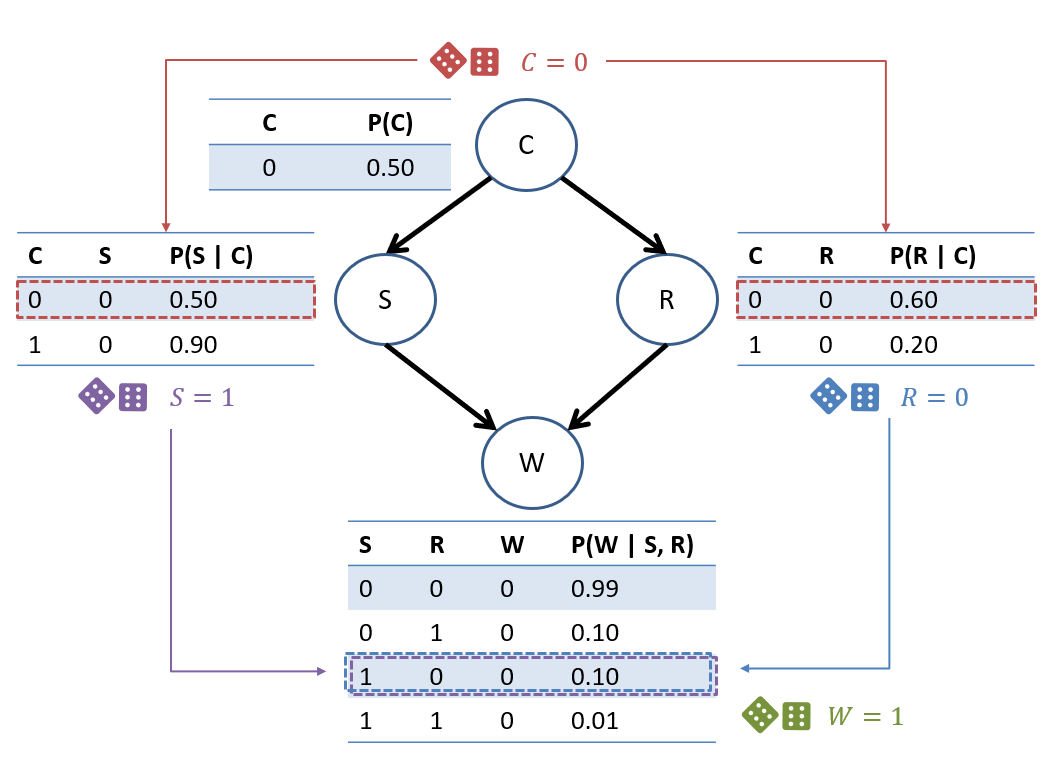
Consider a BN constructed on 4 binary variables: \(C\) = whether or not it's cloudy; \(S\) = whether or not there are sprinklers on; \(R\) = whether or not it's raining; \(W\) = whether or not the sidewalk is wet.
God that example is boring... but does it ever get results!
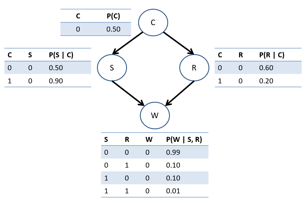
Example parameters stolen shamelessly from Berkeley's CS 188 materials (with permission).
Suppose we then generate the following samples, i.e., simulated outcomes for each variable knowing the network parameters, ignoring for the moment how we *got* them:
Sample |
C |
S |
R |
W |
|---|---|---|---|---|
0 |
1 |
0 |
1 |
1 |
1 |
1 |
1 |
1 |
1 |
2 |
0 |
1 |
1 |
0 |
3 |
1 |
0 |
1 |
1 |
4 |
0 |
0 |
0 |
1 |
Q1: Examining the table above, how would we estimate \(P(W=1)\)?
Simply count the number of samples in which that's true and divide by the total number of samples!
So, since we have 5 samples, and in 4 of them \(W = 1\), we would estimate the value of this query to be: $$\hat{P}(W=1) = 4/5 = 0.80$$
Note the cute hat over the \(P\) above; this notation is generally used to distinguish the "real" distribution \(P\) from a sampled estimate \(\hat{P}\)
Simple! But, how about some conditional queries?
Q2: How about estimating \(P(C = 1 | W = 1)\)?
Since the evidence is \(W=1\), we ignore any sample in which that is not the case, and then look at the proportion of times \(C=1\) in those that remain!
Above, since sample 2 has \(W = 0\), we would ignore it in pursuit of computing this query, and would find that, in the remaining 4 samples, \(C=1\) 3 times, meaning we'd estimate. $$\hat{P}(C = 1 | W = 1) = 3/4 = 0.75$$
Neat!
Note: there's an inherent tradeoff between the speed of generating just a few samples, and the accuracy of generating many.
To get a gist for just what kind of computational effort has to be invested in sampling, let's think about means of actually using a BN and then generating a sample like the one above.
Prior Sampling
Brainstorm: given the BN structure and semantics (viz., CPTs in form of each node given its parents), what would be a reasonable way to generate samples from a BN?
You likely were able to brainstorm a couple of key insights:
Each variable's likelihood depends on the value of its parent(s)
For any given sample, we can generate values for the parents first, and then roll biased dice for the value of the children based on their conditional likelihood.
This technique is called Prior Sampling, which relies on sampling network variables by order of a topological sort.
A topological sort of a directed graph is an ordering of nodes in which a node never appears before all of its parents already have in the sequence.
Using a topological sort ensures that we never sample a child node before we know the value of its parents in the sample.
In our example Rainy Sidewalk network, there are a couple of viable topological sorts:
\(C, S, R, W\)
\(C, R, S, W\)
Although not unique, either one of these will suffice. Without loss of generality, let's see how we might create a sample using the first:
Sample Order, \(i\) |
Previously-sampled Givens |
Variable, \(V\) |
\(P(V = 0 | Pa(V))\) |
\(P(V = 1 | Pa(V))\) |
Example Sample of \(V_i\) |
|---|---|---|---|---|---|
\(0\) |
\(\{\}\) |
\(C\) |
\(0.5\) |
\(0.5\) |
\(C = 0\) |
\(1\) |
\(\{C=0\}\) |
\(S\) |
\(0.5\) |
\(0.5\) |
\(S = 1\) |
\(2\) |
\(\{C=0,S=1\}\) |
\(R\) |
\(0.6\) |
\(0.4\) |
\(R = 0\) |
\(3\) |
\(\{C=0,S=1,R=0\}\) |
\(W\) |
\(0.1\) |
\(0.9\) |
\(W = 1\) |
Depicted, the process above would look like:
Simple, intuitive, and generates a consistent sample... but in simplicity, there is some opportunity for improvement.
What are some problems with Prior Sampling for estimating posterior queries like \(P(C | S = 0)\)?
Irrelevant Samples: if the desired query is a posterior like \(P(C | S = 0)\), we may generate many samples for which \(S=1\) due to the topological ordering, which need not have been generated to begin with.
Idea: how about we short-circuit any sample that is inconsistent with the query's evidence?
An enhancement to Prior Sampling is known as Rejection Sampling by which any sample inconsistent with evidence is immediately ignored / thrown out.
Although this improves our efficiency a bit, and is consistent in the limit for conditional probabilities, we can imagine that there's a better way to go about it.
Suggestion: Suppose, in order to answer \(P(C | S = 0)\), we simply fix \(S = 0\) and then perform Prior Sampling on the other variables -- would this technique be consistent?
Not in general! Why? Because knowledge about \(S\) provides "upstream" evidence about \(C\) that would not be captured by the topological nature of Prior Sampling!
So, it would seem, we need some stronger tools to think about how to efficiently answer conditional queries.
Gibbs Sampling
To recap:
Prior sampling is fine if our queries are on joint or marginal quantities, but can be innefficient for posterior / conditional queries.
We can't simply fix any evidence in a conditional query and then perform Prior Sampling because fixing a variable as evidence may make upstream variables dependent on that information.
To formulate a new approach to address the above, let's make one crucial insight:
Insight 1: Sampling from some variable \(V\) given *all other* variables in the network is much easier than sampling from the JPT itself!
Suppose, for example, we wanted to sample \(S\) given all other variables, viz., \(P(S|C,R,W)\). We have:
\begin{eqnarray} P(S|C,R,W) &=& \frac{P(S, C, R, W)}{P(C, R, W)} \\ &=& \frac{P(S, C, R, W)}{\sum_s P(s, C, R, W)} \\ &=& \frac{P(C) P(S|C) P(R|C) P(W|S,R)}{\sum_s P(C) P(s|C) P(R|C) P(W|s,R)} \\ &=& \frac{P(C) P(S|C) P(R|C) P(W|S,R)}{P(C) P(R|C) \sum_s P(s|C) P(W|s,R)} \\ &=& \frac{P(S|C) P(W|S,R)}{\sum_s P(s|C) P(W|s,R)} \\ \end{eqnarray}
Notice: many factors from the Markovian Factorization cancel out!
Insight 2: To sample from a variable given all other variables, we need only the CPTs that mention the one being sampled!
Consolidation: if we fix all variables in the network except for one being sampled, the computation is easy and still takes any observed evidence into consideration.
The procedure for taking advantage of these insights is a simple one known as Gibb's Sampling:
Gibbs Sampling is a method for efficiently sampling posterior queries \(P(Q | e)\) consisting of the following steps:
Initialize all variables to some random assignment, except for the evidence \(e\) which remains fixed to its value.
Sample a single variable at a time conditioned on the rest (again keeping \(e\) fixed).
Repeat Step 2 many times.
Intuitively, this process both takes observed evidence into consideration, and allows it to provide information about other variables being sampled while still allowing the sampling to be computed efficiently.
Let's look at an example!
Consider sampling \(P(S | R = 1)\) (depicted as \(P(S | +r)\) in the graphic below):
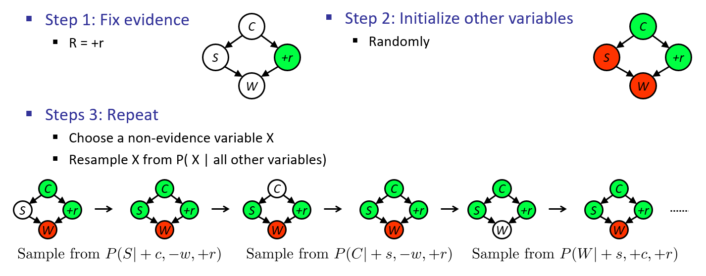
Graphic stolen shamelessly from Berkeley's CS 188 materials (with permission).
Here's that same network but ANIMATED Gibbs' Sampling! (this time: by yours truly).

Neat! Some notes on the above:
When we resample a variable \(X\) in in step 3.2 above, we will do so for each variable \(X_i\) in the BN exactly once to generate a *single* sample of the format \(\langle X_0, X_1, X_2, ... \rangle\).
The next sample at iteration \((t+1)\) will use the initial state of the variable values sampled at iteration \((t)\).
Because the first samples begin from the random assignment in Step 2, they are often innacurate and discarded up to some defined "burn-in period" number of samples.
Just to concrete what we mean when we say to "sample from" the distribution of a single variable in the sequence above:
What is the likelihood that we sample \(S=0\) given that \(C=1, R=1, W=0\) in the first step shown above?
$$\begin{eqnarray} P(S=0|C=1,R=1,W=0) &=& \frac{P(S=0|C=1) P(W=0|S=0,R=1)}{\sum_s P(S=s|C=1) P(W=0|S=s,R=1)} \\ &=& \frac{0.9 * 0.1}{0.9 * 0.1 + 0.1 * 0.01} \\ &\approx& 0.99 \end{eqnarray}$$
Pretty dang certain we sample \(S=0\) for that first step!
So there you have it! Approximate inference in all of its glory -- we'll make use of these tools in another context soon!