Reasoning Over Time and Space
Thus far, one of our fundamental assumptions about Bayesian Networks and Probabilistic Reasoning has been that evidence is collected for a single quantum, or state frozen in time.
Why might this be limiting in some capacity? Where might we gain some opportunities to refine our probabilistic inference capabilities?
We should be able to meaningfully combine observations across different time periods or locales in order to increase the accuracy of our inferences.
List some examples of when concerting sequences of observations over time / space might be useful.
A player's moves in a board / card game with partial information
Monitoring someone's blood pressure over time / medical applications
Speech recognition (phonemes form words when combined over time)
Meteorological predictions
In fact, it's often *very* important to be able to concert information gathered over time.
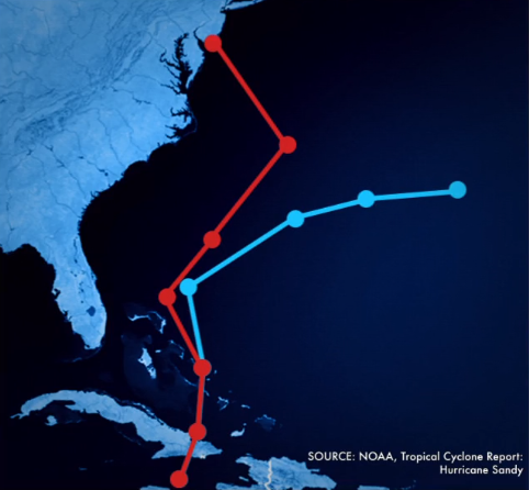
Consider the semi-recent meteorological predictions of Hurricane Sandy's path into the continental US, in which the US weather model predicted it hanging wide out to sea (blue in image below) and the EU model correctly predicted it impacting the mainland (red in image below).
Plainly, this is a skill that humans use often as well, as many aspects of prediction require not only the ability to discern multiple past observations, but to use those to predict future events as well.
Today, we'll start that journey by marrying some of our probabilistic models into the ability to reason over time.
Markov Models
Let's start by thinking about a simple, motivating problem, and finally one that actually makes some measure of sense given the context...
Take a weather forecast system that can use the weather's state on any given day to provide information about the predicted weather on the next.
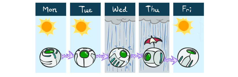
Adorable cartoon borrowed from Berkeley's AI materials, with permission.
Intuition: why might reasoning over time be useful in forecast generation?
Basic human intuitions that rain is typically followed by more rain (depending on locale, of course), BUT after so many days of rain, we expect it clear up.
How can we formalize situations like this, perhaps in terms of some probabilistic reasoning tools recently discussed?
Trace the likelihoods of variables over slices of time in which *state* has some likelihood of *transitioning*
From these intuitions, we can develop what are known as (and yes, he's back) Markov Models:
Markov Models / Markov Chains model the changes in some State Variables over slices of time / space as specified by Transition Probabilities (AKA Dynamics).
The transition probabilities are assumed to be stationary such that the likelihoods of state transition are the same at each quantum of time.
The stationarity assumption is vital lest our Markov Models have absolutely no predictive power: if the likelihoods that states change are themselves changing over time (at least in some unforeseeable way), then we can't really make any claims as to what the state will be in the future.
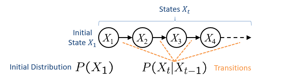
Graphically, Markov Models will look like a familiar friend:
Let's get some binding of our intuitions to some of the formalisms implicit above:
Why don't we draw arrows from earlier states to ones that are more than one state away? E.g., why not draw an arrow from \(X_1 \rightarrow X_3\)?
For two reasons: each node represents the state at some time slice, and since the transitions exhibit stationarity, the next state is *only* reliant on knowledge of the previous and the transitions.
The Markov Property in Markov Chains (same as in Bayesian Networks) provides a nice property (and philosophy): The future is independent of the past given the present.
Bask in that thought for one second: "It doesn't matter how you got here, it only matters where you go next."
And that brief moment of reflection, friends, is why this class is satisfying one of your Core Flags. Whew! On to the good stuff...
In particular, the Markov Property allows us factor the joint distribution of these state variables over time very conveniently:
In a Markov Chain with a time horrizon \(T\) and initial state \(X_1\), the joint distribution over all states at time \(t \in T\) can be expressed: \begin{eqnarray} P(X_1, X_2, ..., X_T) &=& P(X_1) P(X_2 | X_1) P(X_3 | X_2) ... P(X_T | X_{T-1}) \\ &=& P(X_1) \prod^{T}_{t=2} P(X_t | X_{t-1}) \end{eqnarray}
Of course, we don't want to recreate the entire joint distribution over multiple time slices, but rather, use our Markov Models to answer questions about specific \(P(X_t)\).
However, computing an arbitrary \(X_t\) means knowing the distribution over state values of \(P(X_{t-1})\).
As such, we can apply a recursive definition to compute an arbitrary future state that we'll call the Mini-Forward Algorithm.
The Mini-Forward Algorithm provides the ability to simulate the transition propagation such that, for any arbitrary future time slice \(t\) we have: \begin{eqnarray} P(X_t = x_t) &=& \sum_{\text{Prev state possibilities}} \text{\{Transition probability\}} * \text{\{State likelihood at previous\}} \\ &=& \sum_{x_{t-1} \in X_{t-1}} P(X_t = x_t | X_{t-1} = x_{t-1}) P(X_{t-1} = x_{t-1}) \end{eqnarray}
Numerical Example
Using the Markov Property, let's see how this applies to a simple, numerical example.
Suppose that \(X = \{rain, sun\}\) and the weather is sunny today (i.e., \(P(X_1 = sun) = 1\)); what is the likelihood that it will be sunny in 2 days (i.e., find \(P(X_3 = sun)\))?
Assume also we have the following transition probabilities, which can be equivalently stated in either CPT or state-diagram format:
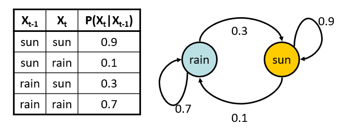
Example parameters stolen shamelessly from Berkeley's AI materials, with permission.
So, to solve for \(P(X_3 = sun)\), we can apply the Mini-Forward algorithm from the initial state to the desired one, starting with solving for \(P(X_2)\):
\begin{eqnarray} P(X_2 = sun) &=& \sum_{x_1} P(X_2 = sun, X_1 = x_1) \\ &=& \sum_{x_1} P(X_2 = sun | X_1 = x_1) P(X_1 = x_1) \\ &=& P(X_2 = sun | X_1 = sun) P(X_1 = sun) + P(X_2 = sun | X_1 = rain) P(X_1 = rain) \\ &=& 0.9 * 1.0 + 0.3 * 0 \\ &=& 0.9 \\ \therefore P(X_2 = rain) &=& 0.1 \end{eqnarray}
Not a surprising result! When we started with certainty, we would expect the day following that certainty to be equivalent to the transition probability... but if we wanted to peer *farther* into the future, we would need to repeat the process.
Now, to find our query, we apply it once more:
\begin{eqnarray} P(X_3 = sun) &=& \sum_{x_2} P(X_3 = sun | X_2 = x_2) P(X_2 = x_2) \\ &=& P(X_3 = sun | X_2 = sun) P(X_2 = sun) + P(X_3 = sun | X_2 = rain) P(X_2 = rain) \\ &=& 0.9 * 0.9 + 0.3 * 0.1 \\ &=& 0.84 \\ \therefore P(X_3 = rain) &=& 0.16 \end{eqnarray}
For most Markov Chains, repeated application of the Mini-Forward algorithm yields what is known as the Stationary Distribution, which marks the point at which no future application of the algorithm will change belief about the next state.
For example, it turns out the stationary distribution for the example above is denoted \(P(X_\infty)\) and ends up being pretty tidy:
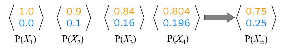
Example parameters stolen shamelessly from Berkeley's AI materials, with permission.
There are some interesting theoretical consequences of the stationary distribution, including in application to web-relevance for search engines.
We won't be discussing those here, but they're worthy of further inquiry!
That's all we have to say about these basic Markov Models -- next time, we add some twists!