Reasoning over Time (Continued)
Last time we discussed Markov Models (MMs) as useful tools for modeling an agent's ability for reasoning-over-time.
However, whereas MMs represent *ideal* scenarios wherein the State Variables (X) we care about are observed, we should take a step back and consider a more realistic setting:
More often than not, rather than observing the State Variables (X), we observe noisy sensors of X known as emissions.
Consider some scenarios wherein the state, which may change over time, can only be witnessed through noisy proxies.
[Robotics] Where a robot is in a room (state) as it moves may be indicated by noisy range sensors (emissions).
[Health] Progress of a stroke (state) may be indicated by worsening symptoms (emissions) like slurred speach.
[Nature] Impending earthquakes (state) may be indicated by changes in underground electromagnetic activity or animal movements (emissions).
As such, a shortcoming of basic Markov Models is that it is difficult to separate state from emission... so let's do that now!
Hidden Markov Models (HMMs)
We have some assumptions about what we'll want to model in a more general format of MMs:
State is still changing over time / space, but its direct observation is not possible for the agent.
Emissions are observations that emanate *from* the current state.
We want to use all observed emissions up until the current time \(t\) to make assessments about the next state.
Defining HMMs
To accomplish the above, we'll tweak our definition of Markov Models in a simple, but powerful way.
A Hidden Markov Model (HMM) assumes an underlying Markov Model that is not observed, but in which emissions, or output evidence *from* the underlying Markov Model, is observed.
Graphically, an HMM looks like:
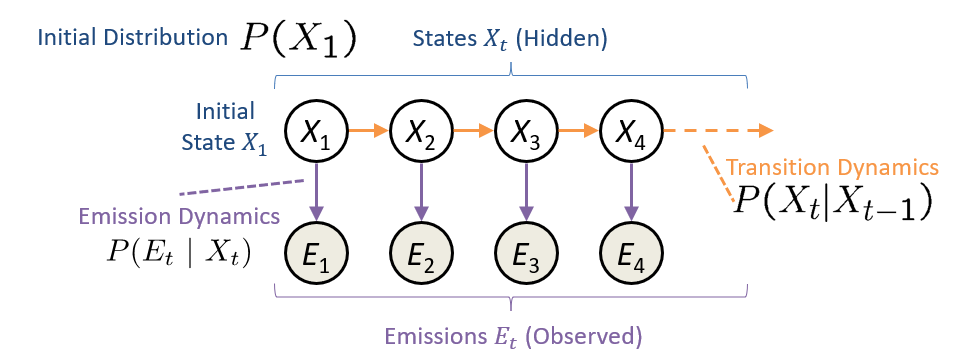
Notably highlighted above are the three key components that we define in an HMM:
\(P(X_1)\), the likelihood of each value in the initial state.
\(P(X_t|X_{t-1})\), the transition likehoods for the hidden state between time steps.
\(P(E_t|X_t)\), the likelihoods of each observed emission given the state.
Where would we typically get all of these?
The initial state distribution usually begins as the uniform distribution (i.e., equal chance of being in any state).
The transition likelihoods might be gathered from past, longitudinal data on the state.
The emission likelihoods might be based on known sensor innaccuracies, or again, past data.
With the foundation set, let's examine some new and exciting properties of HMMs.
Properties of HMMs
Let's begin with how the joint distribution can be factored using our HMM template above, assuming we have only states and emissions up until time \(t=3\):
$$P(X_1, E_1, X_2, E_2, X_3, E_3) = P(X_1) P(E_1 | X_1) P(X_2 | X_1) P(E_2 | X_2) P(X_3 | X_2) P(E_3 | X_3)$$
This gives us a general formula for factoring an HMM joint:
Generalized HMM Joint Factoring $$P(X_1, E_1, ..., X_T, E_T) = P(X_1) P(E_1|X_1) \prod^T_{t=2} P(X_t|X_{t-1}) P(E_t|X_t)$$
From this generalized factoring, we can make some more important insights. Let's go with my signature Socratic method to expose those:
In an HMM, does the Markov Property still hold? Namely, are future states \(X_{t+i}\) independent of past states \(X_{t-j}\) given the present \(X_t\)?
Yes! A simple examination of the network structure reveals this through the rules of d-separation.
What's the practical challenge with the Markov Property in an HMM?
We never observe the state! It's what's hiding from us... sneaky sneaky state!
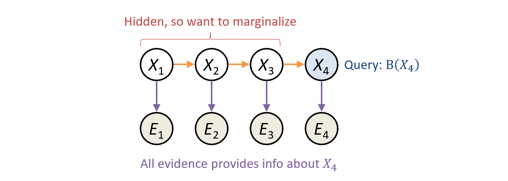
As a consequence of never directly observing the state, all past evidence / emissions becomes relevant for predicting the hidden state at any given time.
This is simple to verify if, for example, we're trying to assess the state \(X_3\): is \(X_3 \stackrel{?}{\indep} E_1\)? \(X_3 \stackrel{?}{\indep} E_2\)?
As such, we need some approach that, given all collected evidence, can concert their information about the state we want to predict.
Filtering
Though helpful to think about the decomposition of the joint distribution theoretically, difficult to use it practically, especially as inferences about our desired state \(X_T\) with many observed \(e_1, e_2, ..., e_T\) trend farther into the future.
We can think instead about tracking the distribution as it evolves over time through a process called filtering:
Filtering (AKA monitoring) describes the process of tracking and updating a belief state \(B(X_t)\) over time where: $$B(X_t) = \text{Belief of state of X_t given all past evidence} = P(X_t | e_1, e_2, ..., e_t) = P(X_t | e_{1:t})$$
This is, after all, our chief goal: we want to estimate the likelihood of the state at time \(t\) given all past evidence!
Let's see why this might be useful before examining *how* to accomplish its estimation:
Illustrative Example
Let's look at a neat example that depicts, at a high-level, where we're headed with these tools.
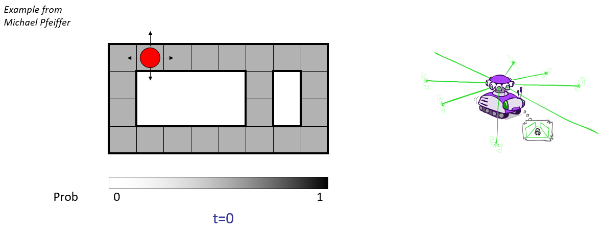
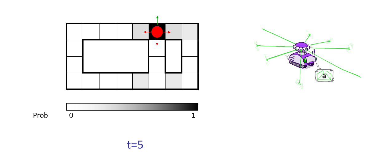
Robotic Navigation: in this "Roomba-like" problem, a robot is navigating a room according to some directional sensors and is attempting to localize its position on some map, with the following:
State: location of the robot in some room / hallway.
Sensor / Emission Model: short range proximity detector that can determine if there's a wall on any of 4 sides, but is a noisy reason; will never make more than 1 mistake.
Motion Model: can move in any of 4 cardinal directions, but might get stuck (on carpet or something) with some small chance.
Some notes on each step below:
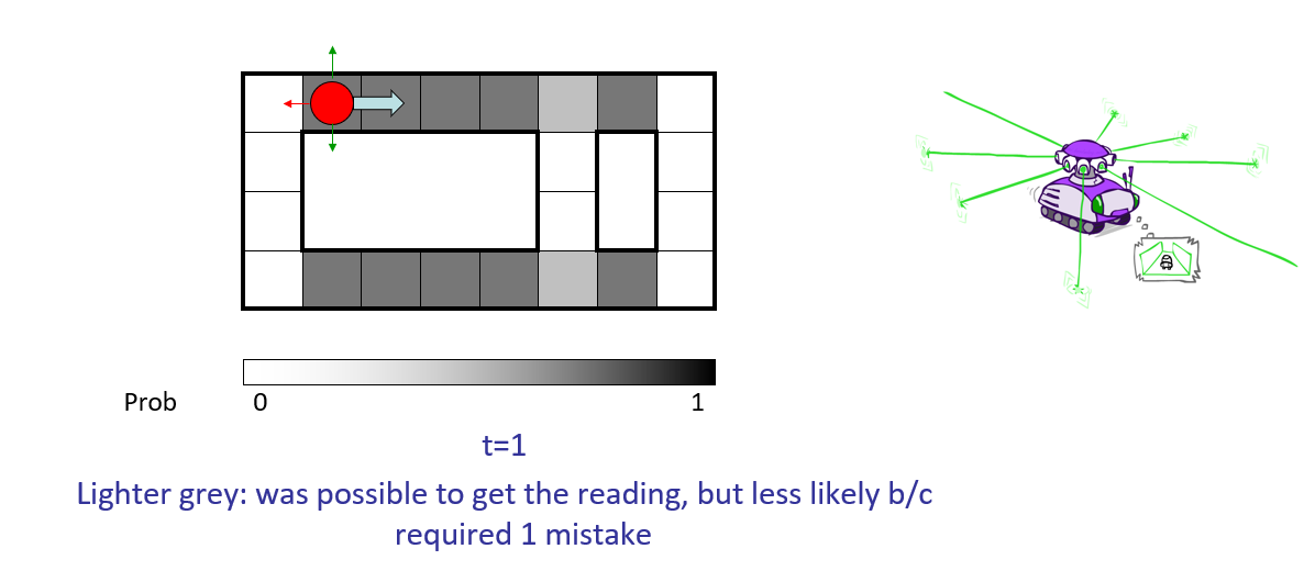
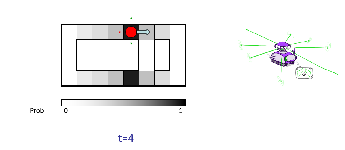
Depicted in each time step as the red dot is the *actual* location of the bot in the room (the hidden state).
The shades of gray in each cell depict the bot's belief that it is in a given state with what confidence; this begins as the uniform distribution (it could be anywhere!) but is updated as we gather observations and elapse time.
Example credit to Berkeley's AI Materials, displayed with permission.
With this motivation in place, let's actually see how we go about performing these time-evidence updates on beliefs.
HMM Inference
Recap: Inference in HMMs is akin to determining the belief of the state at some time: $$B(X_t) = P(X_t | e_{1:t})$$
What are the challenges associated with computing some arbitrary belief state \(B(X_t)\)?
Primarily, we need to find an efficient means of:
Accounting for what all previous transitions and evidence up until time \(t\) tell us about \(X_t\)
Marginalizing / Summing over all possible values of the hidden states.
Let's see how we might go about doing this...
\begin{eqnarray} B(x_t) &=& P(x_t | e_{1:t}) \\ &\rightarrow& \text{using conditioning, we can normalize later, let's focus on the numerator} \\ &\propto& P(e_{1:t}, x_t) \\ &\rightarrow& \text{using law of total prob., sum over previous state \(x_{t-1}\)} \\ &=& \sum_{x_{t-1}} P(e_{1:t}, x_t, x_{t-1}) \\ &\rightarrow& \text{break the \(e_{1:t}\) term apart at the previous state's evidence} \\ &=& \sum_{x_{t-1}} P(e_t, x_t, x_{t-1}, e_{1:t-1}) \\ &\rightarrow& \text{repeated use of conditioning (aka, chain rule)} \\ &=& \sum_{x_{t-1}} P(e_t | x_t, x_{t-1}, e_{1:t-1}) P(x_t | x_{t-1}, e_{1:t-1}) P(x_{t-1}, e_{1:t-1}) \\ &\rightarrow& \text{simplifying via HMM structural independence} \\ &=& \sum_{x_{t-1}} P(e_t | x_t) P(x_t | x_{t-1}) P(x_{t-1}, e_{1:t-1}) \\ &\rightarrow& \text{rearranging and noting that \(P(x_{t-1}, e_{1:t-1}) = \alpha B(x_{t-1})\) for normalizing \(\alpha\)} \\ &=& P(e_t | x_t) \sum_{x_{t-1}} P(x_t | x_{t-1}) * \alpha B(x_{t-1}) \\ &\rightarrow& \text{intuitively:} \\ &=& \text{{emission dynamics}} * \sum_{\text{all possible last states}} \text{{transition dynamics}} * \text{{belief of being in last state}} \end{eqnarray}
This final result, viz.: \begin{eqnarray} B(x_t) &=& P(e_t | x_t) \sum_{x_{t-1}} P(x_t | x_{t-1}) P(x_{t-1}, e_{1:t-1}) \\ &=& P(e_t | x_t) \sum_{x_{t-1}} P(x_t | x_{t-1})~\alpha~B(X_{t-1}) \end{eqnarray} ...for normalizing constant \(\alpha\) provides the roadmap for our solution in what is known as the Forward Algorithm.
Forward-Algorithm Intuition: "Push" belief states from earlier time states forward such that if we knew \(B(X_{t-1})\), we could use that as a "checkpoint" through which to compute \(B(X_t)\).
Although the Forward Algorithm gives us a nice roadmap for a solution, it's difficult to imagine implementing it programmatically unless we broke it apart into some pieces more amenable to traditional programming practices...
Given the above recursion for finding \(B(x_t)\) based on \(B(x_{t-1})\), what kind of an algorithm might we deploy here?
Dynamic programming! Solve the big problem from earlier recurrences / applications of the forward algorithm.
To make this dynamic programming component simple, we can think of decomposing the Forward Algorithm down into two repeated update steps:
Computing \(B(X_t)\) follows repeated application of two steps at all previous time steps:
Passage of Time: Update the belief for the transition / time between \(X_{t-1} \rightarrow X_{t}\). Namely, define: $$\color{green}{B'(x_t)} = P(x_t | e_{1:t-1}) = \sum_{x_{t-1}} P(x_t | x_{t-1}) \color{red}{B(x_{t-1})}$$
Observation: Update for observed emission for time \(t\): \(X_{t} \rightarrow E_{t}\). Namely, define: $$\color{red}{B(x_{t})} = P(x_t | e_{1:t}) \propto P(e_t | x_t) \color{green}{B'(x_t)}$$
Note: the derivations of the above update rules are a bit handwavy, though you can see where they come from in the Forward Algorithm.
Interested in a fuller proof? Click here!
Deriving the Update Rules
Note: lots of subscripts and proofiness awaits you here -- read on if you want to see the nitty-gritty of how we get the above!
Rule 1 - Updating for Time: intuitively, computes the likelihood of being in the next state \(X_{t+1}\) given all evidence \(e_{1:t}\) by weighting our belief that we were in the previous state \(B(x_t)\) by the likelihood of each transition \(P(X_{t+1}|x_t)\) $$P(X_{t+1} | e_{1:t}) = \sum_{x_t} P(X_{t+1}|x_t) P(x_t|e_{1:t}) = \sum_{x_t} P(X_{t+1}|x_t) B(x_t)$$
Compactly, we represent this quantity as \(B'(X_{t+1})\): $$B'(X_{t+1}') = \sum_{x_t} P(X_{t+1}'|x_t) B(x_t)$$ ...where the parameter \(X_{t+1}'\) is the same in the weighting \(P(X_{t+1}'|x_t)\)
In the Update for Time, we computed: $$B'(X_{t+1}') = P(X_{t+1} | e_{1:t})$$ If we now acquire a new emission evidence for time \(t+1\) we must estimate: $$P(X_{t+1}|e_{1:t+1})$$
Since that's not something we have immediately available, let's see if we can factor it:
\begin{eqnarray} P(X_{t+1}|e_{1:t+1}) &=& \frac{P(X_{t+1}, e_{1:t+1})}{P(e_{1:t+1})} \\ &=& \frac{P(X_{t+1}, e_{t+1}, e_{1:t})}{P(e_{t+1}, e_{1:t})} \\ &=& \frac{P(X_{t+1}, e_{t+1} | e_{1:t}) P(e_{1:t})}{P(e_{t+1} | e_{1:t}) P(e_{1:t})} \\ &=& \frac{P(X_{t+1}, e_{t+1} | e_{1:t})}{P(e_{t+1} | e_{1:t})} \\ \end{eqnarray}
Now, here's some magic... since the only purpose of that denominator is to normalize the result, and does not depend on our query \(X_{t+1}\), let's just "proportion" it away:
\begin{eqnarray} P(X_{t+1}|e_{1:t+1}) &\propto& P(X_{t+1}, e_{t+1} | e_{1:t}) \\ &=& P(e_{t+1} | X_{t+1}, e_{1:t}) P(X_{t+1}|e_{1:t}) \\ &=& P(e_{t+1} | X_{t+1}) P(X_{t+1}|e_{1:t}) \\ &=& P(e_{t+1} | X_{t+1}) B'(x_{t+1}) \end{eqnarray}Note that since \(B(X_t) = P(X_{t}|e_{1:t}) \Rightarrow B(X_{t+1}) = P(X_{t+1}|e_{1:t+1})\), so, finally, we get:
$$B(X_{t+1}) \propto P(e_{t+1} | X_{t+1}) B'(x_{t+1})$$
WHEW! All that just to get our query into a format we could compute from the model's transitions and emission dynamics!
We now have our second rule:
Rule - Updating New Observation: intuitively, computes the likelihood of being in the next state \(X_{t+1}\) given some NEW evidence \(e_{t+1}\) on top of all existing evidence \(e_{1:t}\), and after accounting for passage of time \(B'(X_{t+1})\): $$B(X_{t+1}) \propto P(e_{t+1} | X_{t+1}) B'(x_{t+1})$$
Note! The above states only a proportional-to operation, so we must renormalize after every cycle of updating for observation!
We can think of these two general steps as implementing the human feedback loop: try closing your eyes and walking forward...
With Passage of Time, certainty about your environment diminishes (you'll lose track of where you are if you keep walking blind!).
With Updates for Observation (if you were to open your eyes briefly), certainty about your environment spikes / sharpens.
These are precisely the types of processes that HMMs are meant to model; uncertainty from passage of time, and certainty from evidence in a constant loop!
Numerical Example
The part you've all been waiting for!
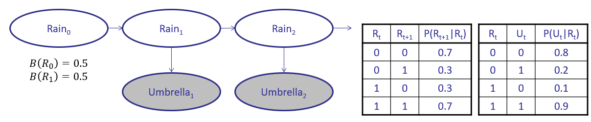
You've been stuck in Keck with the blinds drawn for close to 3 days now, blithe to the weather outside. Still, you decide to use some inference to determine the likelihood of whether or not it's raining outside, given that you've seen people come in with umbrellas the past 2 days. In other words, find \(P(R_2 = 1 | U_1 = 1, U_2 = 1)\)
We'll use the HMM specified below to answer this question:
Step 1 - Setup and Priors: we'll be completing the following table in classic dynamic-programming fashion, with the base-case of our belief over the initial state, sans evidence:
\(t = 0\) |
\(t = 1\) |
\(t = 2\) |
|
|---|---|---|---|
Time Update: \(B'(R_t)\) |
- |
||
Observation Update: \(B(R_t)\) |
\begin{eqnarray}B(R_0 = 0) &=& 0.5 \\ B(R_0 = 1) &=& 0.5 \end{eqnarray} |
As stated earlier, it's typical to initialize our prior belief with a uniform distribution over the starting state -- we don't know anything at the start!
Step 2 - Update for Time: compute: $$\color{green}{B'(x_t)} = P(x_t | e_{1:t-1}) = \sum_{x_{t-1}} P(x_t | x_{t-1}) \color{red}{B(x_{t-1})}$$ ...in time-ascending order from what we know (bottom-up dynamic programming).
\begin{eqnarray} B'(R_1 = 0) &=& \sum_r P(R_1 = 0 | R_0 = r) B(R_0 = r) \\ &=& P(R_1 = 0 | R_0 = 0) B(R_0 = 0) + P(R_1 = 0 | R_0 = 1) B(R_0 = 1) \\ &=& 0.7 * 0.5 + 0.3 * 0.5 \\ &=& 0.5 \end{eqnarray}
In general, we'd have to do this for all values of the state, but since it's binary here, we can also assume that \(B(R_1 = 1) = 1 - B(R_1 = 0) = 0.5\)
Using this update for time, we now account for the evidence at the first time slice, namely, that we saw people with umbrellas:
We thus update our table:
\(t = 0\) |
\(t = 1\) |
\(t = 2\) |
|
|---|---|---|---|
Time Update: \(B'(R_t)\) |
- |
\begin{eqnarray}B'(R_1 = 0) &=& 0.5 \\ B'(R_1 = 1) &=& 0.5 \end{eqnarray} |
|
Observation Update: \(B(R_t)\) |
\begin{eqnarray}B(R_0 = 0) &=& 0.5 \\ B(R_0 = 1) &=& 0.5 \end{eqnarray} |
Step 3 - Update for Observation: compute: $$\color{red}{B(x_{t})} = P(x_t | e_{1:t}) \propto P(e_t | x_t) \color{green}{B'(x_t)}$$ ...in time-ascending order from what we know (given the added evidence at each time step).
\begin{eqnarray} B(R_1 = 0) &\propto& P(U_1 = 1 | R_1 = 0) * B'(R_1 = 0) = 0.2 * 0.5 = 0.1 \\ B(R_1 = 1) &\propto& P(U_1 = 1 | R_1 = 1) * B'(R_1 = 1) = 0.9 * 0.5 = 0.45 \end{eqnarray}
Note: the above values are not normalized; if we wanted to report the intermediary steps as actual probability values, we could do so here, but it doesn't matter if we normalize now or at the end.
Still, let's normalize to make things super clear:
\begin{eqnarray} B(R_1 = 0) &=& 0.1 / (0.1 + 0.45) = 0.182 \\ B(R_1 = 1) &=& 0.45 / (0.1 + 0.45) = 0.818 \end{eqnarray}
Updating our table again:
\(t = 0\) |
\(t = 1\) |
\(t = 2\) |
|
|---|---|---|---|
Time Update: \(B'(R_t)\) |
- |
\begin{eqnarray}B'(R_1 = 0) &=& 0.5 \\ B'(R_1 = 1) &=& 0.5 \end{eqnarray} |
|
Observation Update: \(B(R_t)\) |
\begin{eqnarray}B(R_0 = 0) &=& 0.5 \\ B(R_0 = 1) &=& 0.5 \end{eqnarray} |
\begin{eqnarray}B(R_1 = 0) &=& 0.182 \\ B(R_1 = 1) &=& 0.818 \end{eqnarray} |
Step 4 - Repeat! We'll keep doing steps (2) and (3), building our solution up, until we have our final answer.
Left as an exercise: find out how the table is completed in this way:
\(t = 0\) |
\(t = 1\) |
\(t = 2\) |
|
|---|---|---|---|
Time Update: \(B'(R_t)\) |
- |
\begin{eqnarray}B'(R_1 = 0) &=& 0.5 \\ B'(R_1 = 1) &=& 0.5 \end{eqnarray} |
\begin{eqnarray}B'(R_2 = 0) &=& 0.373 \\ B'(R_2 = 1) &=& 0.627 \end{eqnarray} |
Observation Update: \(B(R_t)\) |
\begin{eqnarray}B(R_0 = 0) &=& 0.5 \\ B(R_0 = 1) &=& 0.5 \end{eqnarray} |
\begin{eqnarray}B(R_1 = 0) &=& 0.182 \\ B(R_1 = 1) &=& 0.818 \end{eqnarray} |
\begin{eqnarray}B(R_2 = 0) &=& 0.117 \\ B(R_2 = 1) &=& 0.883 \end{eqnarray} |
Thus, our final answer is in the lower-right-hand cell. Some things to note about the above:
Notice how we construct our solution from previously computed sub-solutions -- bread and butter dynamic programming!
Notice also how the Passage of Time Update from \(t = 1 \rightarrow t = 2\) made us less certain about the rain status...
...but the Observation of the Umbrella at \(t = 2\) sharpened that certainty