Particle Filtering

That's some cool math meets computer science we got up in that previous lecture on HMMs! But...

Let's address the elephant in the room...

Consider the Pacman Ghostbusters example wherein the state is a grid containing the possible locations of the invisible ghost. In a small, 3x3 grid, we might have the following belief state:

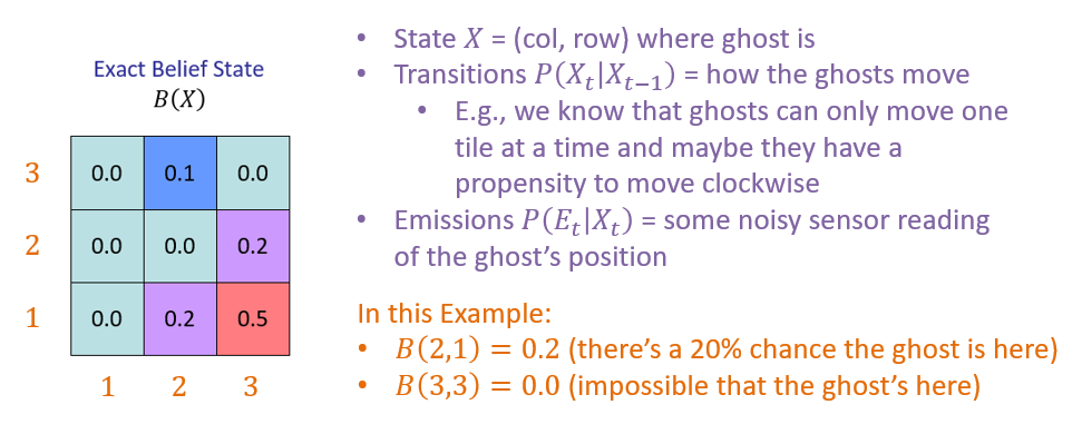
What are some, perhaps, impractical aspects with Filtering for some realistic states $X$?

As the state becomes large (or is continuous, rather than discrete), it can become (1) untennable to store all the different beliefs $B(X)$, and even if so, (2) the likelihoods can become too small for floating point estimates.

In the past, we faced a similar problem with computing exact inference queries on huge Bayesian Networks. What was our solution in that scenario, and how might we generalize that to our current one?

Previously, we used sampling to estimate some probabilistic query -- and we'll adapt that idea to our Hidden Markov Models by developing a new type of sample!

Particles

Approximate Inference in HMMs can be accomplished by representing the belief state $B(X)$ as a list of $N$ particles, which are samples of $B(X)$ that aggregate around the most likely states.

You can consider particles as Votes for the "true" state -- the more votes a state gets, the more likely it is to be the true one!

Suppose we represented our Pacman Ghosthunter belief state from before now with $N=10$ particles.

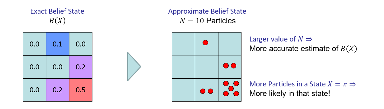
Image ammended from Berkeley's AI Materials, with permission.

So, reasonably, you might ask: how do we actually *use* these particles now that we've defined them as approximate representations of the belief state?

How do we use particles to reason over time in HMMs?

Update their position through the Time Elapse and Observation mechanics just like before!

Now, however, as opposed to simpling reweighting all possible values of the belief state through passage of time and observation, we sample the possible positions of each particle over time!

This describes the new process of Filtering strictly in terms of particles, giving us, unimaginatively...

Particle Filtering Steps

Particle Filtering approximates the Filtering process in 3 steps: Elapsing Time, Observing Evidence, and Resampling, described in detail below.

Step 1 - Elapse Time: Sample the next state of each particle from the transition model $P(X_{t+1} | x_{t})$ such that for particle $x$ we have: $$x_{t+1} = sample(P(X_{t+1} | x_{t}))$$ Note: this means that each particle may move / change its state / vote due to the transition dynamics!

Think of particles as motes of dust floating in the wind (more from my creative writing seminar); most will go in the direction of the wind, but some may spiral and veer off -- the majority that went in the wind's direction give you a good indication for the actual state of the wind.

This step is akin to prior sampling wherein, given the "parent" of the next state in the transition model (the current state), we compute the likelihood of the particle transitioning to some other state.

Let's track the fate of one particle in our Ghostbusters example, as time elapses and it transitions from location (3,3) to (3,2) (highlighted in green below).

Image ammended from Berkeley's AI Materials, with permission.

Note: the above represents our estimate of $B'(X)$ from the exact inference material -- the pre-observation update for passage of time!

After these transitions have taken place on a per-particle basis, we now have the slightly trickier task of updating our approximated belief state once we observe some evidence.

Once we have transitioned each particle through passage of time, and now receive some evidence $e$ that may make some of the particle states *less likely* than others, how shall we update our estimate?

Weight the likelihoods of each particle by their posterior likelihood from the emission dynamics!

Step 2 - Observing Evidence: After observing evidence $e$, downweight each sample based on the emission dynamics such that, for each particle $x$, we assign some weight $w$: $$w(x) = P(e|x)$$ ...due to the result from before that: $$B(X) = P(e|x)*B'(X)$$

What this leaves us with is the same set of samples but with relative likelihoods of each of them given the most recent evidence.

Back to Ghostbustin', consider that we observe evidence that the ghost is close to (3,2) (highlighted in red), which should reweight the likelihoods of each particle based on the emission dynamics (visually, by the relative size of each dot representing each particle).

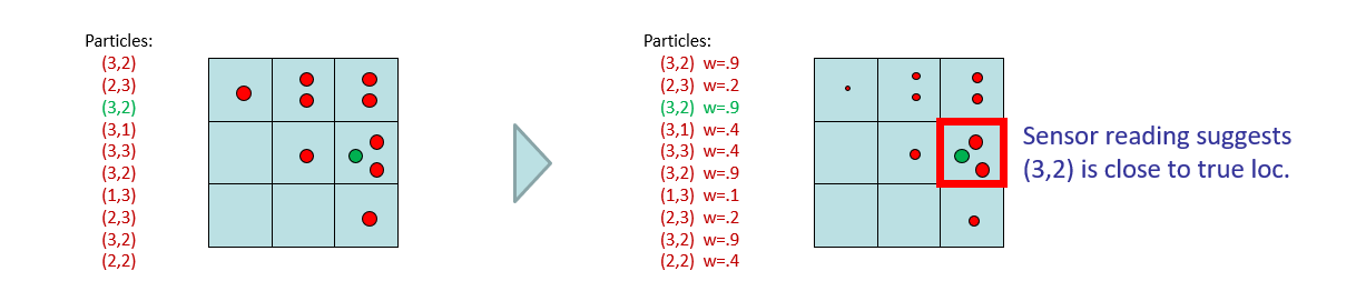
Image ammended from Berkeley's AI Materials, with permission.

Some notes on what we're left with above:

The weights do not sum to 1, plainly, because we never renormalized.
We don't necessarily want to track each particle moving forward because some become very unlikely given their transition and update for observations.
We also don't want to just delete the unlikely particles since then we start slowly chipping away at our value of $N$, losing accuracy as the process continues.

Is there some happy-compromise that solves all of the above?

Simply resample each particle from the weighted particle distribution! This generates a new set of particles that are consistent with the approximate distribution from the previous set.

Step 3 - Resample: For all $N$ particles in the filter, sample a new particle (with replacement) drawn from the weighted distribution found in Step 2.

When we say "with replacement," we mean that we're not necessarily picking up a particle in the pre-resampling phase and moving it into another spot in the post-resampling phase, but rather, using the static distribution in the pre-resampling phase through which we generate new particles in the post.

Once more, in our Ghostbusters example, this appears like:

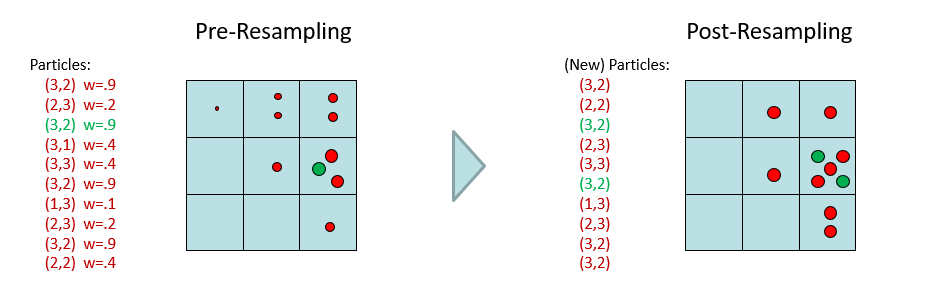
Image ammended from Berkeley's AI Materials, with permission.

The effects of resampling:

The distribution is effectively renormalized without having to compute any gory normalizing constants!
Unlikely particles from the Observation update step are converted into more likely ones while preserving our sample size.

With repetition, the idea is that the majority of particles collapse onto or near a single state, thus performing our inference for us!

Step 4 - Repeat! At this point we're basically back at Step 1 but for time $t+1$ -- we can repeat as long as our agent is online collecting evidence!

Numerical Example

Ghostbusting?! What an impractical example, we should get some practice with something far more realistic!

Reconsider the whether prediction HMM in which the state $R \in \{0, 1\}$ (the weather, rain or sun, respectively) is unknown, but for which we observe the emission $U \in \{0, 1\}$ of whether or not people are using umbrellas.

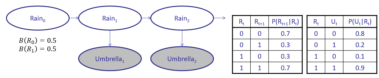
Suppose we wish to use $N=5$ particles to estimate $B(X_1)$, and observe that $U_1 = 1$ (people have umbrellas) and start with the following configuration:

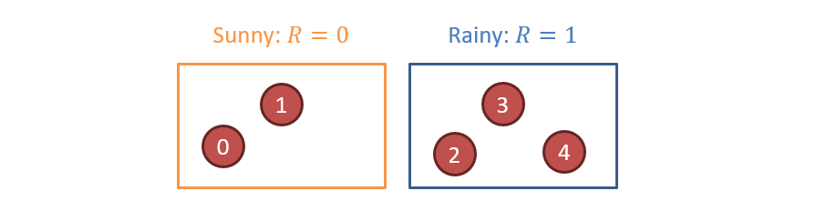
Step 1 - Elapsing for Time: $$x_{t+1} = sample(P(X_{t+1} | x_{t}))$$

What's the likelihood that particle 1 stays in state $R=0$?

$P(R_{t+1} = 0|R_t = 0) = 0.7$, so very likely that it stays where it does!

What's the likelihood that particle 3 moves to state $R=0$?

$P(R_{t+1} = 0|R_t = 1) = 0.3$, so unlikely to change.

Here is an example of how each particle might have moved at this step (remember, when we sample, we are the mercy of the random number generator, so this is just one of other likely configurations):

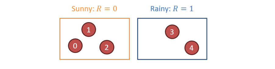
Note: Each of the particles had a chance to move in the above, but the RNG decided that only #2 did.

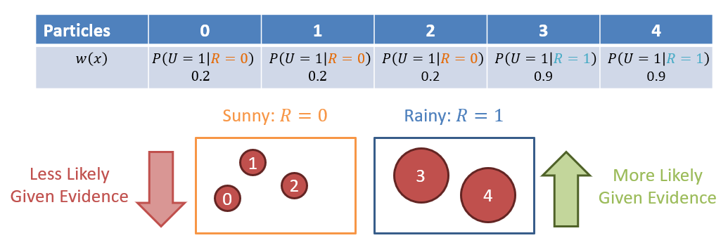
Step 2 - Observing Evidence: Observing umbrellas: $U_1 = 1 \Rightarrow w(x) = P(U_1 = 1|x)~\forall~x \in X$

Observing that people are using Umbrellas means that we should more heavily weight the samples that are consistent with rain, per the emission dynamics $P(E_t|X_t)$.

Step 3 - Resample: For all $N$ particles in the filter, sample a new particle (with replacement) drawn from the weighted distribution found in Step 2.

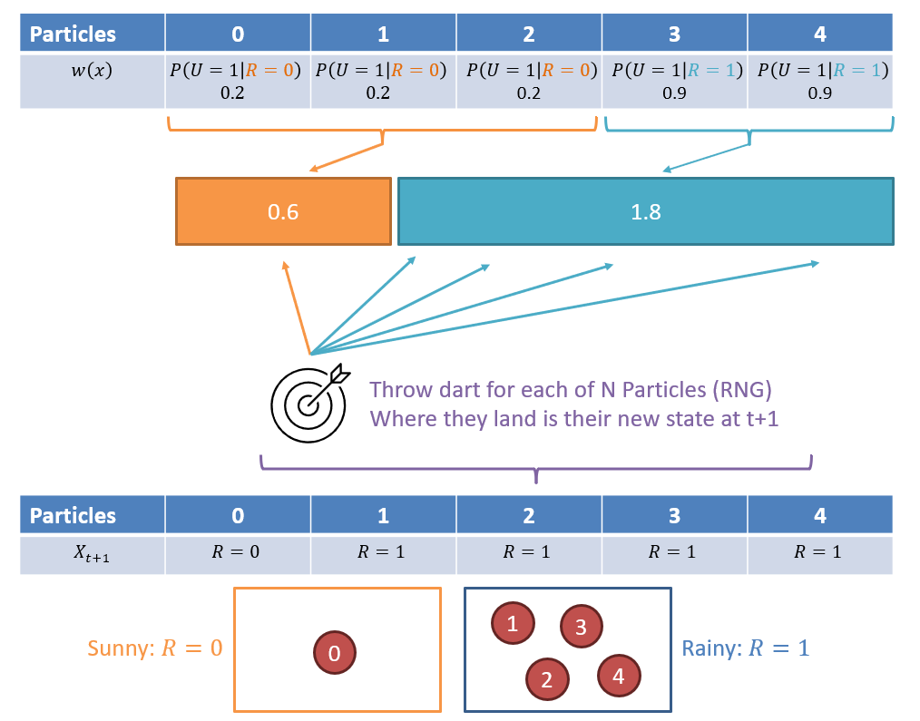
As such, in the above, $B(R_1 = 0) = 1/5 = 0.2, B(R_1 = 1) = 4/5 = 0.8$ -- not a bad estimate from our exact inference, and with only 5 particles!

Real-World Example

It turns out that Particle Filters are used in actual robotic navigation and localization.

Here's an example of particle filtering used in a robotic exploration task -- observe how the particles collapse as the robot moves and its sensor accrue evidence:

Gif credit to Dieter Fox.

Interested in other examples? Check out SLAM: Simultaneous Localization and Mapping used in more advanced robotic exploration systems, which still use some particle filtering!

For now, however, that's all we've got to say about HMMs!