Introduction

Welcome to CMSI 2130: your window into the wonderful world of algorithms!

Course Outline

For those of you viewing from home, at this point we'll review the class syllabus, located here:

Site Structure

Before we get started, some things to note about these course notes and the site you're currently viewing:

You can add notes inside the website so that you can follow along and type as I say stuff! Just hit SHIFT + N and then click on a paragraph to add an editable note area below. NOTE: the notes you add will not persist if you close your browser, so make sure you save it to PDF when you're done taking notes! (see below) Having said that, know that there is a lot of research that suggests taking hand-written notes to be far more effective at memory retention than typing them.
The site has been optimized for printing, which includes the notes that you add, above. I've added a print button to the bottom of the site, but really it just calls your printer functionality, which typically includes an option to export to PDF.
The course notes listed herein will have much of the lecture content, but not all of it; you are responsible for knowing the material you missed if you are absent from a lecture.

Any time you see a blue box with an information symbol (), this tidbit is a definition, factoid, or just something I want to draw your attention to; typically these will help you with the conceptual portions of the homework assignments.

Any time you see an orange box with a cog symbol (), this tidbit is a useful tool in your programming arsenal; typically these will help you with the concrete portions of your homework assignments.

Any time you see a red box with a warning symbol (), this tidbit is a warning for a common pitfall; typically these will help you with debugging or avoiding mistakes in your code.

Any time you see a teal box with a bullhorn symbol (), this tidbit provides some intuition or analogy that I think provides an easier interpretation of some of the more dense technical material.

Any time you see a yellow question box on the site, you can click on it...

...to reveal the answer! Well done!

With that said, let's jump right into it!

Problem Solving

Since this course is about algorithms, let's start by making sure we're all on the same page!

Forward

What is an algorithm?

A formalized procedure for accomplishing some task.

Pretty basic! In fact, you might argue that everything you've been studying in the major thus far has been a study of algorithms -- and you'd be right!

So what makes this class different?

Herein, we study a variety of algorithm paradigms that provide prototypical algorithm formats that can be applied to a wide variety of applicable tasks.

Think of algorithmic paradigms like architectural styles -- no two Romanesque buildings are the same, but share components in common that solve a particular problem (e.g., desired appearance, available materials, etc.)

These paradigms generally have a focus on solving large problems that would be computationally intractible without doing something clever -- the heart of computer science!

In class, we'll see some sample problems that each paradigm is useful for solving, but you should understand that these specific examples are only instances of problems that can be solved by the strategies, which will apply to many others we won't see in 2130 as well.

With that said, let's look at our first paradigm with regards to generalized problem solving.

Beginning Example

If you like puzzles, this class is for you! How about one of the most basic puzzles that many of us spent our childhoods solving on restaurant placemats to pacify us while our parents ate?

In the classic Grid World, some agent starts at a given position in a grid, and our job is to find some path that navigates to some goal cell.

Here's a toy example we'll use to motivate things in class:

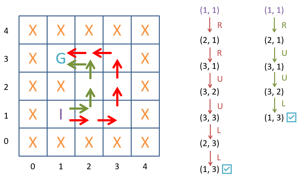
If our agent can move Up, Down, Left, or Right, note some solutions to this problem with the paths above.

Note that there are multiple solutions in the search space to the above -- some that might be considered more *optimal* than others.

The abstract set of possible solutions to a problem its search space, which different search strategies will navigate with their own pros and cons.

Let's see how to formalize this problem, and then look at some search strategies that address problems formalized in such a way.

Formalizing Search

Combinatorial Search (or just Search for short) is the study of algorithms that attempt to solve problems with large search spaces (e.g., problems with many possible solutions or few that are hard to find).

Here's a fun app to play with that shows us just what we're after:

Maze Pathfinder App

Algorithms that procedurally *find* a solution from amongst these possibilities will be at the center of this first portion of the class!

Some areas of search belong to the study of artificial intelligence, but can be applied to so many other tasks that we will give this topic a solid treatment in 2130.

Formalize the problem / components (to know, concretely, what its pieces should look like to a program)
Search for a solution in the search space to the input problem through some procedure
Execute a found plan of action that solves the problem (if one exists at all!)

Just how we define the problem, environment, and actions available to our search algorithms will be of first concern for us.

Formally, a search problem consists of 5 specified components, detailed below (see Roman Numerals, I, II, III, ...).

States are a given instantiation of a search problem's variables of interest, which are liable to change as the agent acts.

I. An initial state is the state at the start of the problem.

II. A goal test / state determines if the state represents a solution to the problem.

An intermediary state is a state between the initial and goal states, as would be encountered during search.

What might a state look like in our motivating problem? What would the initial and goal states look like?

How about the agent's position on the board? The initial state is the cell they begin within (1, 1) and the goal is the position of the goal (1, 3).

III. Actions are the set of choices available to the agent at a state such that $$actions(state) = \{ a_1, a_2, ... \}$$

What can our agent do to manipulate the state? When is are some actions applicable and when are they not?

Move Left, Right, Up, or Down! Not applicable when such a movement would move them into a barrier.

IV. Transition Model specifies how an action taken by the agent in some state leads to some nextState, or formally:
$$transition(state, action) = nextState$$

This makes sense since, if our state is the agent's position, then when they move, they modify the current state of the problem.

How does an action manipulate / transition the state in our example?

Without loss of generality, transition(state, action) = move((x, y), "Up") = (x, y+1), etc.

The set of all possible states that can be reached from the initial state via valid actions is called the state space.

What is the state space in the problem above?

All of the open tiles, including the goal!

V. Costs specify the cost of a particular transition such that for some numerical cost constant $c$, $$cost(state, action) = c$$

What would be a reasonable cost to associate with each of our transitions in the example problem?

Associate a cost of 1 for each valid movement.

When every transition in the problem has the same cost, we call this a uniform cost problem.

Uniform cost problems are easier to solve than non-uniform cost, for reasons we'll see shortly, but for our initial thrust into this domain, we can consider that every action takes the same amount of "effort" to accomplish.

We can depict the above on our Maze Pathfinding Problem as formalized via a search problem.

What are some other types of problems that a formalization like the above could solve?

Recall that this harkens back to our idea of an algorithmic "paradigm" -- being able to apply the same "template" of solution to different specific problems.

Some examples include:

Solving a Rubix cube (and many other types of puzzles).
Finding the best route for a car to take in traffic.
Types of Planning wherein steps must be followed in a specific order (e.g., baking a pie or changing car oil)

Remarkably: if you can formalize a problem into the above components, you can use the following strategies to solve them!

Let's think about what that might look like and how we'd choose from amongst different strategies.

Formalizing Search Strategies

Now that we've defined a problem, we need a means of actually using our carefully laid-out definitions!

Search can be thought of as a function that takes in a problem specification, and returns a sequence of actions that transition the initial state into the goal state, if it exists: $$search(problem) \Rightarrow solution$$

In our motivating Maze Pathfinding example, what would a solution look like?

A series (i.e., ordered sequence) of actions that lead from the initial to a goal state: $$solution = [a_1, a_2, ..., a_k] = [\text{'U'}, \text{'D'}, ...]$$

Search strategies define a procedural means of finding such a satisfying solution from a formalized search problem.

In the context of Maze Pathfinding, we'll need our search strategies to:

Explore all possible transitions that might lead us to the goal from the initial state (though not more than we need to).
Have some way of remembering the sequence of steps of these possible transitions from start to finish so that a solution can be returned.

Can you think of an appropriate data structure that might be well suited for the purpose of exploring the search space by satisfying the criteria above? Describe its properties.

A tree where the initial state is at the root (or a graph, for reasons we'll discuss later).

A search tree is a companion data structure used in search with the following properties:

Nodes representing states with the initial state at the root.
Edges representing actions leading to the transitional next state nodes.

If a goal is reached through some path from the root, then a solution exists from tracing the path from the root.

Viewing the above start to a search tree, we make a few notes:

We wish to find the optimal (shortest) path even though there are many possible.
We will probably want to avoid repeated states lest we duplicate effort.
We need some procedures for creating the search tree and will focus on how efficient these are.

So, naturally, we should first describe what properties of a solution a search strategy should optimize, and then consider some candidate algorithms:

With these metrics of success in place, let's look at some basic search strategies:

Uninformed Search

Search strategies proceduralize search by the manner in which the search tree is constructed, nodes visited, and how child nodes are generated.

Similar to the tree traversal algorithms we saw in data structures (provided an ordered visit of nodes in the tree), search strategies provide an ordering for constructing a search tree.

A companion data structure used during search strategies to hold unexplored nodes/states is known as the frontier (think about your history classes where the frontier was the edge of known territory!)

Across all strategies, search tree construction happens in repetition of two primary steps, though with some differences at each step:

Expansion: removes a node from the frontier as the next candidate to explore:
```
  expandedNode = frontier.pop()
```
(note: we're using the pop() method generally here, not necessarily meaning the frontier is a stack)
Generation: adds all possible next states from an expanded node to the frontier; this is how we remember where to explore in the future:
```
  for a in actions(expandedNode):
      frontier.add(transition(expandedNode, a))
```

[Data Structures Tie-in] Because we are interested in returning a sequence of actions (i.e., a path) for a solution in the search tree, what should each node record-keep (i.e., what fields should each have)?

Each node in a search tree tracks:

The state the node represents
The parent node that generated it (for recreating the solution path)
The action that generated it (since there may be multiple ways of reaching this state)
[For Non-Uniform Cost Problems] The Path Cost $g(n)$ encountered from the initial state to this node (will be important later)

Here is a search tree where we expand the root, generating its children (assuming each movement is legal), and then expand the child node corresponding to a taken "right" action:

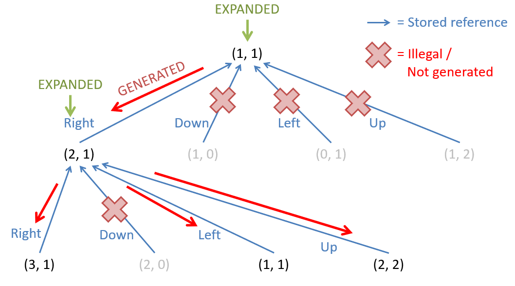
Notes on the above:

The *red* arrows show the direction of node generation from parent to child (i.e., after expanding a parent, and concluding it is *not* the goal, we then generate the children).
The *blue* arrows show the references that each child node remembers of its parent (important for remembering the path that led to it).
Some nodes that would otherwise be generated are not because the action that would have generated them is illegal from the parent's state (viz., those actions are ones that would run you into a wall!)
Pausing the search tree construction at the image above, the leaf nodes $(3,1), (1,1), (2,2)$ would be the nodes stored in the frontier.

Thus far, we've only seen the process of expanding and generating a search tree, but not yet how to actually *use* it to perform search!

Uninformed Searches are strategies that expand nodes simply by some order in which they were generated. These are the simplest strategies that require no problem-specific information to perform.

Important characteristics of uninformed searches:

The stopping conditions (when the search tree construction ends):
1. The goal test yields true for a *GENERATED* node $\Rightarrow$ solution found!
2. The frontier is empty $\Rightarrow$ no solution found!
Importantly from the above: the goal test is performed during generation, not expansion, but this is not true for all search strategies.

Breadth-First Search

We all remember Breadth-First Graph Traversal from data structures, yes? Well it's back to help us grow some trees!

What were the characteristics of breadth-first traversal, and what data structure did we use to accomplish it?

BFS searches "level by level" in a search tree, never expanding a node that is more than 1 level deeper than another. We used a Queue frontier to implement it.

BFS: (FIFO) Enqueue newly generated nodes in the Queue frontier, and expand in dequeued order.

Use BFS to find a solution to our original problem (omit some paths that don't lead to the solution, for ease). Consider that child nodes are generated using the action precedence: Right, Down, Left, Up

Metrics of Optimality

There are two primary metrics of optimality for a search strategy:

The quality of the solution returned.
The efficiency with which it finds it.

Related to the problem definition alone (i.e., trait #1 above), what properties should be true of any solution returned by a good search strategy?

Two of the most important:

Completeness: if a solution exists, the strategy is *guaranteed* to find it.

Optimal Cost: if an optimal (i.e., lowest cost) solution exists, the strategy is guaranteed to return it.

There are also two classic metrics of optimality from a computational standpoint:

What computational metrics of success should we analyze for any given search strategy?

Space and Time Complexity: Some sort of asymptotic bound for the growth of the amount of time the algorithm takes to complete, or the memory that must be allocated to it as a function of the size of the input (or in our case, the search space).

Since we didn't talk about Space Complexity as much in data structures, here's everything you missed:

What's the worst-case asymptotic bound of memory/space required to store $n$ items in any List, Stack, Queue, Priority Queue, Map, or Set?

$O(n)$ because all $n$ insertions (in the worst case) demand their own stored element (even if just a reference to an object).

For example, every time we added a new element to a List, Stack, Set, Map, etc. it grew by 1 (i.e., a constant) element, so all space needs were linear.

This analysis gets a bit more complicated when it comes to search...

Why might the space complexity analysis become non-linear for search operations?

Search trees may require an exponential number of nodes to fully explore the search space while maintaining their completeness and optimality guarantees.

As such, these trees can get pretty big, and we'll need to be clever with them to avoid overgrowth!

There, now you're caught up! (pretty dull, right? tis why we didn't talk so much about it in data structures, but we will now!)

Breadth-first Search Optimality

Let's stop to consider some of our search strategy optimality metrics.

Is BFS complete?

Yes! It is guaranteed to find a solution if one exists, since it will never generate a level that is more than 1 depth greater than the last.

Is BFS optimal?

Yes, *for uniform-cost problems,* because all states on the same depth will share the same cost, and it will find the most shallow goal state.

Now, to answer questions of computational and space complexity, we need some extra descriptives for the search trees we are generating.

Describe some of the important characteristics of a search tree for time and space complexity.

A search tree's branching factor (b) of a search strategy is the maximum number of children a node can generate when expanded.

Note that if the tree's branching behavior is not uniform (i.e., some nodes' expansions generate more children than others), an average branching factor can be computed for certain amortized analyses.

A search tree's depth (d) is the depth of the most shallow goal node.

Consider the example tree below where the values inside each node are the order of expansion in a BFS where children are added to the frontier in left-to-right order. In this problem, we have $b = 2, d = 3$

Notes on the above:

$b=2$ since no node has more than 2 children
$d=3$ since the shallowest goal node is at a depth of 3.

[!] Note: The following assumes that the goal test is performed during Node generation, i.e., that if a goal node is ever generated, the search is complete and a solution returned.

This kind of goal test is performed differently for later search strategies so pay attention to the algorithms that follow!

Let's now consider the time complexity / asymptotic runtime efficiency in terms of $b, d$ in terms of the number of nodes that are expanded and generated:

First, we should characterize the worse case performance: where the goal state is the *last* expanded on a particular level.

Second, let's chart the number of nodes expanded and generated at each depth, then generalize for a depth of $d$:

Tree Level	Nodes Expanded	Nodes Generated	Nodes in Memory
0	$b^0 = 1$	$b^1 = 2$	$b^0 + b^1 = 3$
1	$b^1 = 2$	$b^2 = 4$	$b^0 + b^1 + b^2 = 7$
2	$b^2 = 4$	$b^3 = 8$ Goal would be found during generation here (goal @ $d=3$ found), and search terminated!	$b^0 + b^1 + b^2 + b^3 = 15$ ...but let's consider what would happen for trees with arbitrary depth $d$
d-1	$b^{d-1}$	$b^{d}$	$b^0 + b^1 + ... + b^{d}$

Insights from the table above:

We need to maintain nodes along the frontier *and* previously expanded nodes in memory so that we know the solution when we find it.
In the worst case where the goal test is performed during generation, this makes the total number of nodes generated on a search tree: $b^0 + b^1 + b^2 + ... + b^d$

Asymptotically, how many nodes are generated? Hint: which will be the asymptotically dominant term in the summation above?

$O(b^0 + b^1 + b^2 + ... + b^d) = O(b^d)$

As such, the worst-case time and space complexity of BFS is $O(b^d)$, even though fewer nodes $O(b^{d-1})$ are actually expanded.

Take a second to visualize the behavior of BFS in the PathFinding.js animation linked above!

Graph Search

Observant students will look at the last search tree and remark: some states are repeated in expansion!

This is certainly a computationally costly fault with search-trees. Certainly we can do better.

Will breadth-first search's completeness be compromised by repeated states?

No, because even though some paths are re-explored, any path that eventually leads to a solution will still be discovered because BFS explores along each path 1 action at a time.

Can you suggest an alternative approach that would avoid repeated states?

Search graphs are exactly like search trees, except that performing graph search never re-expands nor generates a previously expanded state.

Functionally, graph search is the same as tree search except:

We maintain a graveyard / closed set of previously expanded states.
Expanding a node adds that state to the graveyard, and these states are never generated again in the future.

Take, for example, our Maze Pathfinding problem wherein we can compare Tree Search (below, left) to Graph Search (below, right) in a BFS exemplified below.

Note: repeated states that have already been expanded need not proliferate the expansion of the tree, as is indicated in the purple edges in the graph that return the search to a previously expanded state.

That said, these are just depictions of the "search graph," though in practice the edges do not exist.

Time for an *animated example* to tie everything together!

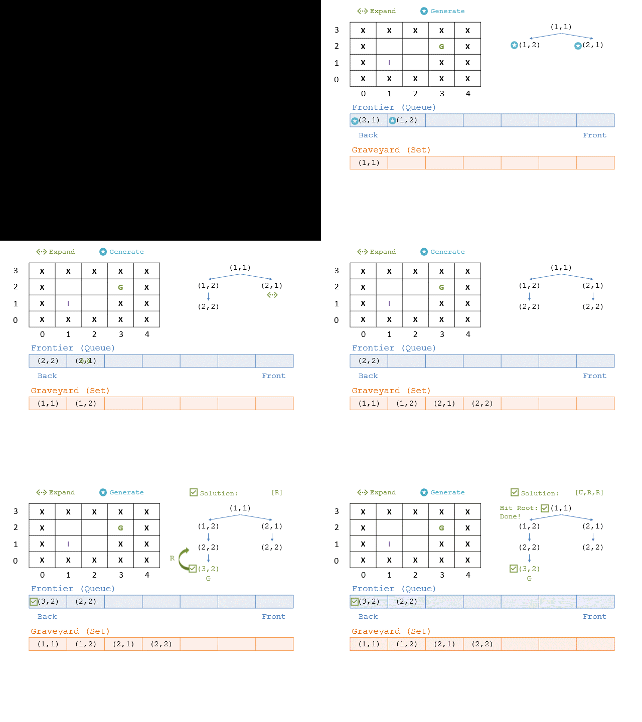
Record-keeping of past effort to avoid repeating effort in the future is a form of a more general paradigm known as memoization / caching that we'll explore more later.

What data structure would well suit the task of memoizing which states have already been expanded in graph search?

In general, a Set (usually, a HashTable implementation), since arbitrary memoization and lookup can be accomplished in $O(1)$. In Maze Pathfinding, there's some argument to be made for a 2D array, but that can be very memory intensive.

Note: memoization can be useful for uniform cost problems, but has strings attached for non-uniform cost problems that we'll talk about later!

Be sure to memoize memoization -- it's an incredibly useful tool to remember!

Of course, we've only looked at BFS for our uninformed search strategies; it's time to examine the merits of another approach...

Depth-First Search

Naturally, if BFS is an uninformed search strategy, we should examine the merits of Depth-First Search as well!

What were the characteristics of depth-first search, and what data structure did we use to accomplish it?

DFS prioritizes "deepest" nodes first in a search tree, always expanding the nodes at the greatest depth first (i.e., the most recently generated). To obtain this behavior, we used a Stack to implement it in data-structures.

DFS: (FILO) Push newly generated nodes onto the Stack frontier, and expand in popped order.

Attempt to use DFS on our example problem in which nodes on the stack frontier are generated in the order of actions $[R, D, U, L]$; what divergent cases can happen?

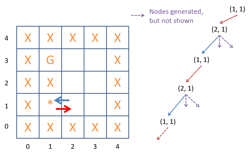
Oh no! We're stuck in an endless expansion loop!

Intuitively, you might say to apply memoization to avoid exploring repeated states just like before, but beware!

There are problems with applying memoization with Depth-First Search:

Since we're searching paths *depth* first, we may accidentally memoize a state in one branch that we *should* be able to explore again on another. As such, memoization applies only on a subtree-basis, and we must be careful to either remove / record separately visited states between subtrees. Failing to do so can compromise completeness or optimality.
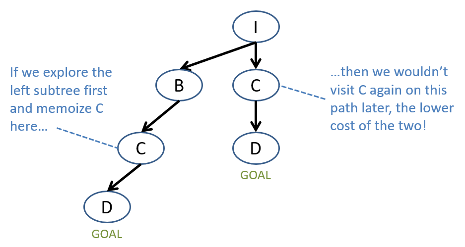
As mentioned above, memoization lands us in hot water for non-uniform cost problems, which we'll see later.

As such, performing memoization naively with DFS can compromise optimality! But, if we're clever with our implementation, we may not need it... and in fact, may find some other performance benefits elsewhere!

To recap:

We need to avoid the infinite expansion pattern like the one above.
We can't use memoization like with breadth-first graph-search.

If we knew the depth of the shallowest goal node, what could we potentially limit to satisfy both of the above?

The depth of generated nodes!

This is behind the motivation for our first realizable implementation of DFS, though not without its own problems...

Depth-limited Search

Depth-limited search is a form of DFS parameterized by some depth threshold $m$ such that the search tree will never generate nodes past a depth of $m$.

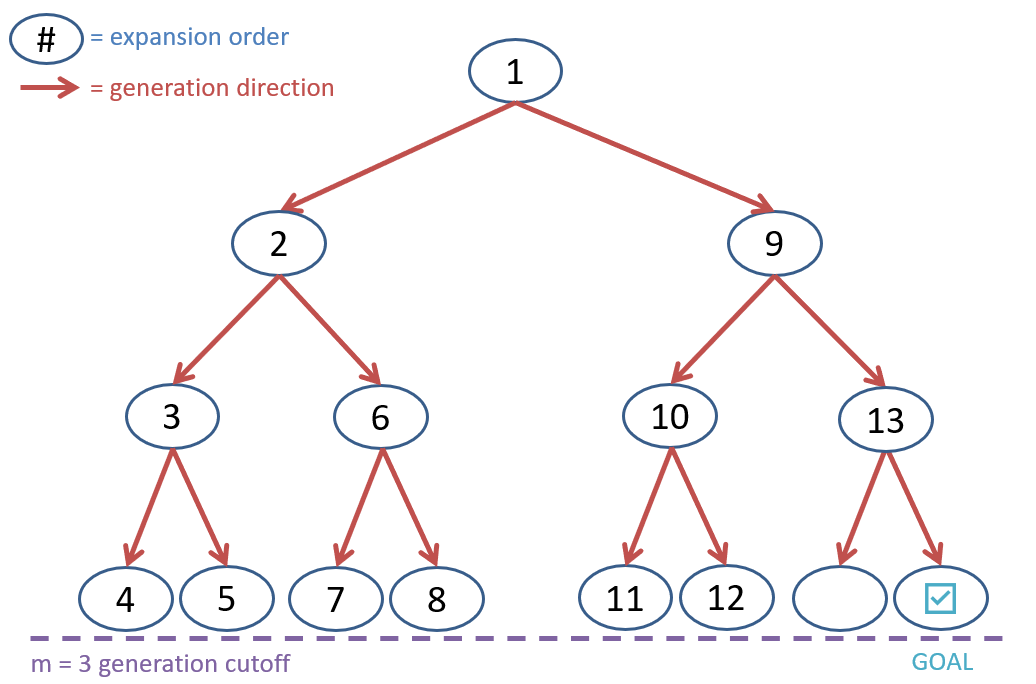
Using depth-limited search, suppose we generated the same abstract search tree as with the BFS example, though (for readability) now add nodes to our Stack frontier in right-to-left order $(b = 2, d = 3, m = 3)$:

Some notes on the above:

We're showing the nodes at the cutoff depth as being expanded to demonstrate the DFS frontier ordering, even though they do not generate any children.
The final 2 nodes generated (level 3, far right) are not expanded because our goal test is still being performed at generation, at which point we'd find the last node as a goal from which to return a solution.
This might look like it's doing more work than the BFS equivalent, but note that we've generated the same number of nodes!

Because we generate the same number of nodes as BFS, we see that the time complexity of depth-limited search is the same, just at our depth cutoff of $m$, giving us $O(b^m)$

Naturally, this begs the question of what depth-limited search even does for us differently than BFS?

To answer this question, we have to dive back to data structures for a moment, and visualize what's happening with our allocated nodes and references that point to them...

Consider that we pause right after expanding node 3 in our depth-limited search above, with nodes A, B, C, D on the frontier.

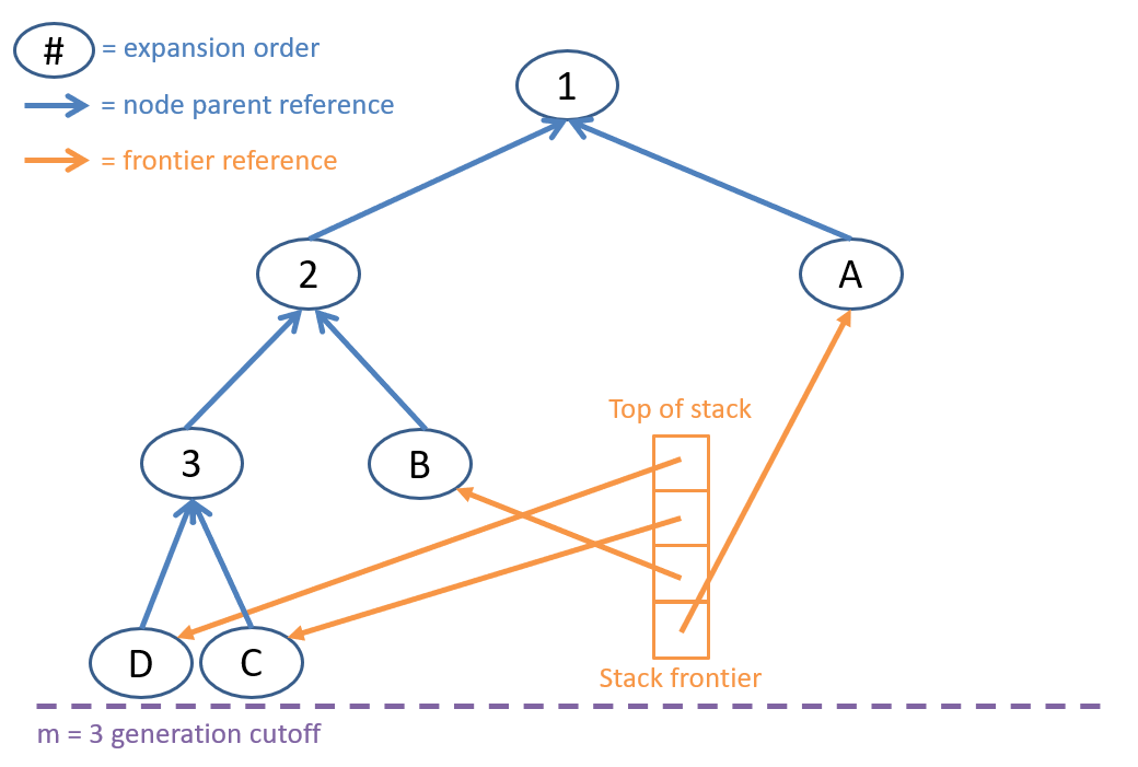
What happens to Node D when it is popped from the frontier, has no children referencing it (as it's at the cutoff), and is not the goal?

It is freed from memory because there are no more references to it!

What happens to Node C when it is popped from the frontier, has no children referencing it (as it's at the cutoff), and is not the goal?

Not only is IT freed from memory because there are no more references to it, but now node 3 is also freed because it has no more children referencing it!

Insight: once a subtree has been expanded fully up until the depth cutoff, and a goal was not found, it is freed from memory!

Consider now that the worst case for the number of nodes held in memory is depicted just above, right after Node 3 is expanded:

Tree Level	Nodes Generated	Nodes in Memory
0	$1$ (special case for root)	$1$
1	$b = 2$	$1 + b = 3$
2	$b = 2$	$1 + b + b = 5$ This is the maximal number of nodes kept in memory before we start freeing nodes!
m	$b$	$1 + b + b + b + ... = O(m*b)$

As such, the space-complexity of depth-limited search is $O(b*m)$, a huge improvement over BFS' exponential $O(b^d)$.

However, there's a problem with depth-limited search as well... what if we don't know $d$, the depth of the shallowest goal?

Depth-limited search may choose an $m \lt d$, and so fail to return a solution (i.e., would be incomplete), or $m \gt d$ and potentially find a goal that was along a non-optimal path (i.e., would be suboptimal)

Is there a remedy to this problem?

Iteratively increase the depth limit until a goal is found!

Iteratively-Deepening DFS (IDDFS)

Iteratively Deepening DFS (IDDFS) performs depth-limited search for $m = 0, m = 1, ..., m = d$ (i.e., until the limit is the same as the goal depth).

Visually, this looks like a depth limit $m$ expanding until a goal is found:

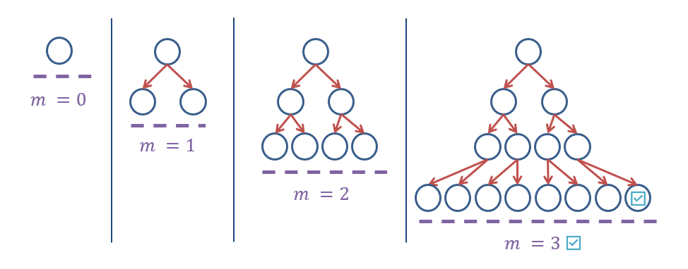
Note! This means that the search tree is *regenerated* at every iteration, i.e., each iteration is an entirely new tree.

That said, will IDDFS have the same time complexity as BFS? Why or why not?

Yes! Because the largest depth explored, $O(b^m) = O(b^d)$ will always dominate the other, smaller search trees explored (asymptotically).

Will IDDFS have the same space complexity as BFS? Why or why not?

No! Because we'll gain the space-saving abilities of DFS to free nodes early in the search, making the worst case $O(b*m) = O(b*d)$.

IDDFS thus preserves the completeness enjoyed by BFS while gaining the space-saving features of DFS, for the small overhead of having to repeat earlier parts of the search.

As such, BFS has a smaller constant-of-proportionality due to the IDDFS overhead of exploring smaller models, but has the same asymptotic runtime.

Punchline: use BFS if all you care about is speed, depth-limited search if you know $d$, and IDDFS if you need more memory!

That brings us to the end of our "dumb" uninformed searches! Next week, we look at... you guessed it... searches that know what's up!

Tree Level	Nodes Expanded	Nodes Generated	Nodes in Memory
0	\(b^0 = 1\)	\(b^1 = 2\)	\(b^0 + b^1 = 3\)
1	\(b^1 = 2\)	\(b^2 = 4\)	\(b^0 + b^1 + b^2 = 7\)
2	\(b^2 = 4\)	\(b^3 = 8\) Goal would be found during generation here (goal @ \(d=3\) found), and search terminated!	\(b^0 + b^1 + b^2 + b^3 = 15\) ...but let's consider what would happen for trees with arbitrary depth \(d\)
d-1	\(b^{d-1}\)	\(b^{d}\)	\(b^0 + b^1 + ... + b^{d}\)

Tree Level	Nodes Generated	Nodes in Memory
0	\(1\) (special case for root)	\(1\)
1	\(b = 2\)	\(1 + b = 3\)
2	\(b = 2\)	\(1 + b + b = 5\) This is the maximal number of nodes kept in memory before we start freeing nodes!
m	\(b\)	\(1 + b + b + b + ... = O(m*b)\)