Thus far, in our formalizations of problem solving and search, we have made some assumptions about the environment that (although may apply to certain restricted problem sets) are not generalizable, and may limit the effectiveness of our approaches.

Moreover, we have been discussing uninformed search strategies...

What made search strategies uninformed?

Search strategies are uninformed when they integrate no problem-specific knowledge or constraints into the search operation.

Our uninformed search strategies are thus "blind" to some problem-specific information that may not only improve runtime performance improvements over those without this information, but can actually lead to more optimal solutions as well!

Recall our search example from last lecture in which we were searching for a path to get our agent to its goal in a grid-world.

Problems with Uninformed Search

---

To wit, suppose our agent must now be able to navigate mud tiles, \(M\) such that the cost of stepping on a mud tile (it's sticky, after all) is 3 rather than the standard 1 for movement onto a regular tile.

Moreover, there may be multiple goals to which our agent can navigate to satisfy the problem (see below).

Consider how our uninformed searches would perform on the above scenario, using the search tree that each might generate:

Above, is the optimal action always the most shallow (i.e., smallest depth) in the search tree?

No! With non-uniform cost problems, this is the case because depth is equivalent to cost (up to some scalar), but not so with non-uniform cost problems.

As such, will any of our uninformed search strategies be optimal?

No! None of DFS, IDDFS, or BFS will be guaranteed to find the optimal solution for non-uniform cost problems.

Problem 1: uninformed search strategies that consider only a set order of expanding nodes may not be optimal for non-uniform cost problems.

We'll have to find a way to take these differing costs into consideration!

That said, let's consider a separate issue: remember our pathfinding animation linked earlier in the week? Observe how wasteful BFS is in finding the route from the initial to goal state.

See all of those tiles that were explored North, South, and West of the initial state? i.e., the ones that were nowhere near closing in on the goal?

These are wasteful explorations and betray the naivety of our uninformed search -- it's simply striking out in all directions without regard for some moves being more likely successes at finding the goal than others.

Problem 2: uninformed search strategies may perform many wasteful explorations that are due to naivety about the problem at hand.

These can be both computationally and memory expensive, and for large search spaces, we want to cut down on both.

Addressing Problem 1: consider how we can empower our search to remain optimal for non-uniform cost problems.

If your intuition was to... I dunno... take the costs into consideration, you're right!

Best-first search strategies expand nodes in order from least- to highest-cost from the initial state.

In this way, we will never expand a node with higher total path cost before one with lower, thus preserving optimality guarantees.

So how do we accomplish this? We need to make 2 tweaks to our existing search strategies:

What extra piece of information will we need to record at each node in the search tree?

The total cost (from the root / initial state) to get to that node, i.e., \(g(n)\) for some node \(n\).

Here, \(g(n)\) for node \(n\) can be intuited as the history / path cost to get to \(n\) from the root and is easily computed by the recursive definition: $$g(n) = g(parent(n)) + cost(parent(n), a)$$ ...where \(a\) is the action that transitioned from \(parent(n) \rightarrow n\).

Note the difference: the \(cost\) is the transition cost, \(g(n)\) is the total cost from the root to that node \(n\).

Of course, having these costs stored in each node is not alone enough to preserve optimality: we now need to incorporate them into our search strategy.

How might we modify our frontier to now expand in order of least- to highest-path-cost?

Make it a priority queue treating \(g(n)\) as the priority!

Warning: re-read that second bullet above! This is different from the uninformed searches we saw last lecture!

Pretty dull evaluation function -- but powerful nonetheless! Let's see it in effect...

Trace the execution of best-first *graph* search on our example below (duplicate states are thus now ignored):

Some notes on the above:

• You should manually verify / step through the \(g(n)\) scores to see where we get the order above.

• Note that an alternative expansion order would have immediately found the optimal goal at expansion 4 instead of 5, though a tie in priority sent us down a small red-herring step on the left subtree at the root.

Will best-first searches now be optimal / complete in non-uniform cost problems?

Yep! Simple proof: we never expand a node (and thus perform a goal-test, which would return the solution) with higher cost than one with lower that's on the frontier.

Yet, we still need to address problem 2: the notion that even best-first searches may still exhibit the same behavior as uninformed searches in exploring many extraneous states.

Addressing Problem 2: consider how we can empower best-first search to omit wasteful explorations during search.

As we saw with our uninformed search strategies, we don't know about any descendants of a particular state (states reachable through some number of legal movements) without first expanding the states in between.

However, just because we don't know what states / costs might be incurred along a certain path, that doesn't mean we can't make educated guesses.

Intuition 1: Note that we obtained optimality on non-uniform cost problems by considering \(g(n)\) the path, or past cost.

Intuition 2: Although search will reveal the optimal solution, we can guide it to be more efficient by estimating the future cost from some node to a goal.

In search, a heuristic is an estimate of cost that is likely to be incurred along a certain path to a solution in the search tree.

Heuristics inform search strategies by providing problem-specific information that can guide the search, leading to more efficient search patterns.

In other words, heuristics represent our best guess for the future cost that would be encountered from a path starting at the evaluated node in a search tree.

For our current maze path-finding problem, what would be a good heuristic that, when given some node \(n\) in the search tree, would estimate how much cost would be incurred on the path to the nearest solution?

We can consider the Manhattan distance heuristic, which would compute the minimal number of movements required to get to the nearest goal from some node.

The Manhattan distance heuristic, parameterized by some node \(n\) in the search tree (given the set of all problem goal states, \(G\)), is functionally defined as: $$h(n) = min_{g_i \in G} |n.X - g_{i}.X| + |n.Y - g_{i}.Y|$$ (Note: the \(min\) operator denotes that the distance returned is for the closest goal \(g_i\) in the set of all goals \(G\))

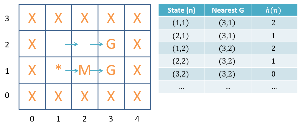
Note: heuristics are just that: rules of thumb! They are not always exact estimates of future cost. The exact costs will be evaluated by the search strategy when it computes \(g(n)\)

Note in the example above wherein \(h((1,1))=2\) though the true future cost will be \(3\).

Give examples for when a heuristic would yield exact vs. inexact estimates of future cost from some node in a search tree.

So how do we implement a heuristic in our Tree Search approach?

If, in best-first methods, we are already recording the history of costs in a node's \(g(n)\), and we have some heuristic \(h(n)\), then what would be a good way to judge the possible merit of a path emanating from some \(n\)?

The sum of the past costs and our estimate for the future ones!

This is precisely the tactic of a widely applied informed search called A* (pronounced "eh-star," like a Canadian astronomer).

A* search is an informed search algorithm by which nodes along the search tree's frontier are expanded according to the result of some evaluation function, \(f(n)\): $$f(n) = Cost_{past}(n) + Cost_{future}(n) = g(n) + h(n)$$ for history cost function \(g(n)\) and heuristic estimate function \(h(n)\)

In words, A* "scores" all nodes along the search frontier according to \(f(n)\) and then expands them in a logical order...

Apropos, if there is some score \(f(n) = g(n) + h(n)\) associated with every node \(n\) along the frontier, what would be a logical order of expansion for A* to perform given that we're interested in finding an optimal solution?

Expand the node with the lowest \(f(n)\), given that it will be our best chance of minimizing cost!

With uninformed searches, we modeled the frontier as a Queue for BFS and Stack for IDDFS, so likewise, we should consider how to implement the desired behavior of A* using a clever choice of data structure.

Because A* is just a variant of best-first search with a new evaluation function / priority for expansion, we can again use a priority queue frontier!

With these implementation details, let's diagram an example run using our troublesome problem for the uninformed searches:

Diagram the A* search tree and found goal state using the problem maze below.

Naturally, the next question for us should be analytical, and investigating the optimality of A*.

Is A* search complete? Is it optimal?

Yes and yes, even for non-uniform cost problems... as long as our heuristic is well chosen.

Visualization

---

Check out the A* visualization here:

Search Visualization

Heuristic Design

---

So what, exactly, constitutes a good heuristic?

Our choice of heuristic for A* search can not only affect its computational performance, but also whether or not it returns an optimal solution!

So, we of course need to vet our choices of \(h(n)\) to determine whether or not they are good implementations of problem-specific knowledge that can aid the search.

What are some desirable traits of heuristics? What must a heuristic never do?

(1) A heuristic must never overestimate the cost to a goal; it should (2) apply problem specific knowledge in pursuit of (3) estimating the true future cost as closely as possible.

Admissibility is a heuristic property required for application to tree search stating that \(h(n)\) will never overestimate the cost of reaching the optimal goal from \(n\).

Why might an inadmissible heuristic compromise the optimality of A*?

An inadmissible heuristic may choose a non-optimal path in the search tree because it may erroneously believe the optimal one to have a cost higher than would be experienced in reality.

For this reason, admissibility is required for guaranteeing optimality for tree search heuristic implementations.

Consider the following search tree and determine why (tracing the execution of A*) the given heuristic is inadmissible.

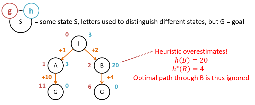
Which of the following are admissible / inadmissible heuristics? For inadmissible ones, provide an example problem that would cause A* to find a suboptimal goal.

  h1(n) = Manhattan distance away from the initial state
  
  h2(n) = (total # of goal tiles) 
        - (# of goal tiles in the same row as n)
        - (# of goal tiles in the same column as n)
        
  h3(n) = Manhattan distance of n from closest goal
  
  h4(n) = # of Mud tiles surrounding n

For A* graph search (i.e., tree search with memoization wherein repeated states are avoided), a slightly stronger (but same idea) criteria is required known as consistency / monotonicity, stating that, for heuristic \(h\), node/state \(n\), next state reached from \(n\) by taking action \(a\), \(n'\), and cost of taking that action \(c(n, a, n')\): \begin{eqnarray} h(n) &\le& cost(n, a, n') + h(n')~\forall n, n' \\ \text{{heuristic estimate to goal from n}} &\le& \text{{cost of taking action a from n to n'}} + \text{{estimate to goal from next state n'}} \end{eqnarray} ...where \(cost(n, a, n')\) is the transition cost from taking action \(a\) in state \(n\) and transitioning to state \(n'\).

This extra criteria is necessary for graph search because if we're never expanding a previously-expanded state, we must ensure that our heuristic would not have a lower future estimate from that repeated next state than from the current one.

Trace the execution of A* GRAPH search in this pathfinding variant below, and determine why an inadmissible heuristic would cause problems.

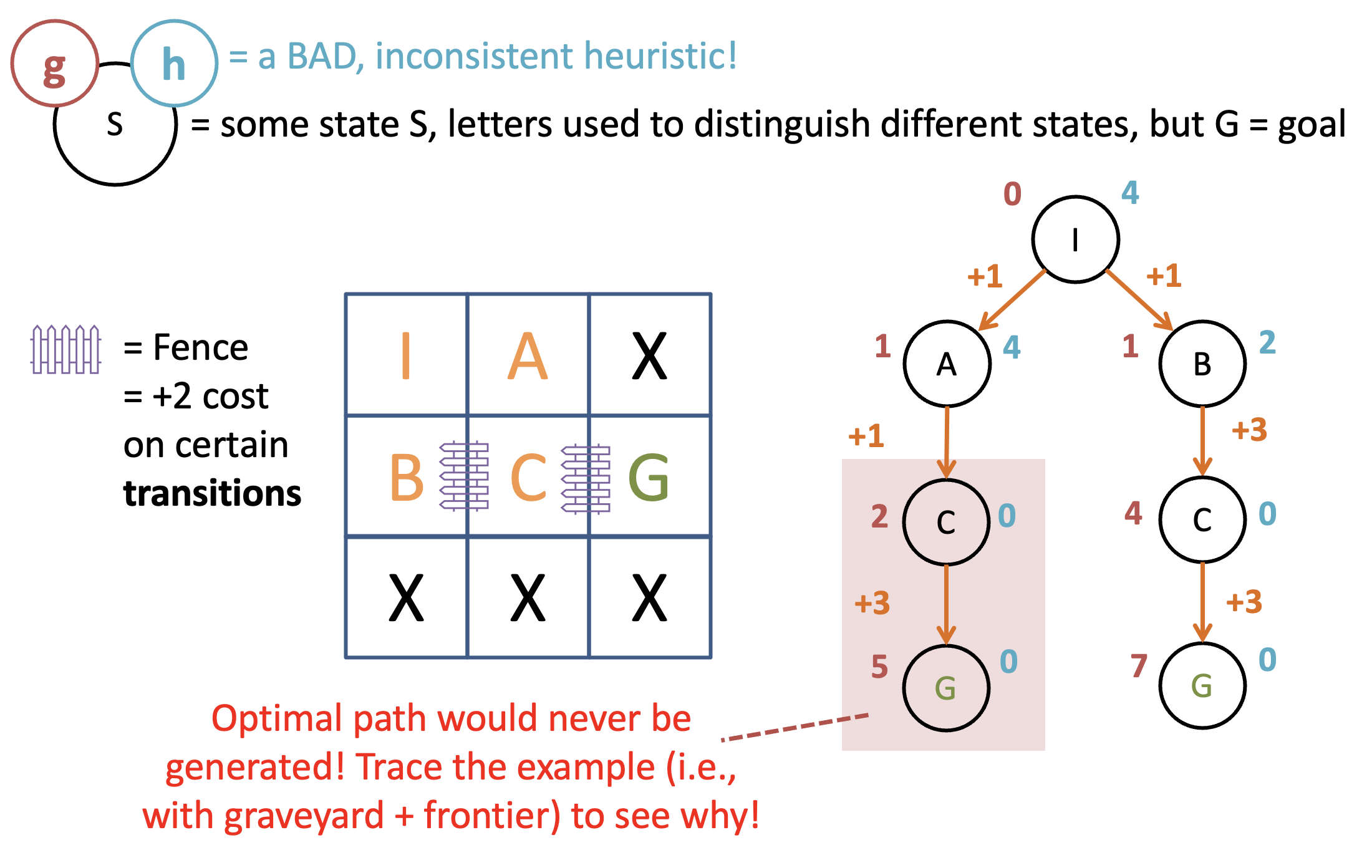
Again, consistency is required to ensure optimality by virtue of never missing a more optimal path due to the order of expansion from A*.

Too abstract? Your coming classwork will have an exercise that makes this clear... just log this one for now!

Plainly, given the above, we see that not all heuristics are created equal -- how, then, can we choose which to use in an implementation of A* and how effective will they be?

Heuristic Efficacy

---

Disclaimer: Heuristic Design is its own subfield of AI, and the below represents only the tip of the iceberg.

We'll look at a few... err... heuristic heuristics now!

First, let's define \(h^*(n)\) as the *TRUE* future cost from \(n\) to the nearest goal.

Why would it be impractical to know \(h^*(n)~\forall~n\)?

Because we would need to perform search from *every* state to determine its optimal future cost!

As such, we may not necessarily have the perfect future estimate, but we do have some guidelines for choosing between heuristics... some heuristic heuristics if you will.

Suppose we have two admissible heuristics \(h_1, h_2\), but \(h_1(n) \ge h_2(n)~\forall~n\). Which should we use, and why?

Prop 1: We should prefer \(h_1\) since it will expand at most as many nodes as \(h_2\), but possibly fewer because it'd be closer to \(h^*\).

However, it's rare that we ever have an admissible that is strictly greater than another admissible heuristic; suppose instead we have a more realistic scenario:

Suppose we have two admissible heuristics \(h_3, h_4\), but \(h_3(n) \not \ge h_4(n)~\forall~n\). How to exploit this scenario to have the best heuristic performance?

Prop 2: Create a third heuristic, \(h_5(n) = max(h_3(n), h_4(n))\). Note: \(h_5(n) \ge h_3(n), h_5(n) \ge h_4(n)\).

Depicted:

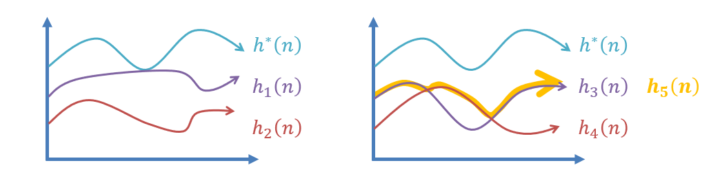
In other words, a heuristic that takes the maximum of two or more other admissible heuristics will always be admissible and fit our first desirable property above.

However, what we have yet to address, is just how to measure how well a heuristic improves performance.

Suppose we *DID* knew the true future cost, \(h^*(n)\) associated with every node to the nearest goal state. How could we evaluate a heuristic's efficacy?

The difference between the true cost and a given heuristics across all states, namely: \(\sum_i h^*(n_i) - h(n_i)\). The larger this sum, the worse the heuristic is.

That said, we also will not be able to evaluate two heuristics across every state as well, whose performance will also vary based on the specific problem instance we are solving.

A more practical approach is to see how a heuristic performs empirically, i.e., across a wide variety of search problems in the same problem space.

To think about how we could assess this empirical performance, we can develop several intuitions:

Intuition 1: The typical empirical means of assessing a heuristic's quality is to measure how much it limits how many nodes were generated.

The more effective the heuristic, the more quickly we get to the optimal solution, therefore the smaller the search tree and thus fewer nodes generated.

However, we would still like an means of quantifying how much of the search tree the heuristic saved us from constructing.

Intuition 2: Our previous computational analyses like on breadth and depth-first search have been more easily considered in the worst case performance for a uniform tree with some branching factor \(b\) and some depth of the found goal \(d\).

A uniform tree is a tree in which each level is full.

Thinking in terms of these uniform trees made performing the asymptotic analysis easy. It'd be nice if we could do that again for the amount of work that a heuristic saves us.

Intuition 3: The optimal goal will be at some depth \(d\), and a heuristic won't change that. It *can,* however, be thought of as reducing the branching factor.

If A* generates \(N\) nodes to find a solution at a depth of \(d\), then the effective branching factor, \(b^*\), is an approximation of the branching factor that a uniform tree containing \(N\) generated nodes and with a depth of \(d\) would have.

\(b^*\) has *no* closed-form solution, but can be found using optimization techniques such that: $$N + 1 = 1 + b^* + b^{*2} + b^{*3} + ... + b^{*d}$$ ...where \(N\) is the number of nodes *generated*, NOT including the root.

To visualize this, let \(n_i\) be the number of nodes generated at level \(i\). In a uniform tree, \(n_i = b^i\). However, this will be less for effective heuristics.

As such, the space and time complexities of A* are \(O(b^{*d})\), though in the worst case, the heuristic is useless at pruning in which case \(O(b^{*d}) = O(b^{d})\)

Since there is not closed-form for computing the effective branching factor, no, I will not require you to compute it on an exam!

Other notes:

• Interestingly, in most problem domains the value of \(b^*\) remains fairly constant despite differences in the individual problems.

• This makes computation of \(b^*\) useful for comparing the efficacy of *different* heuristics on problems.

So now we've seen a variety of different search strategies, and each seems to add something that the last was missing -- why not skip to the end? Did we falter in *pathfinding* our way to A* if it seems like the most capable?

Well, remember that there's no such thing as a free lunch -- getting more adaptive strategies usually come at some costs, and it's all about picking the right tool for the right job -- there are times that you want a jackhammer vs. just a regular old hammer you swing.

Apropos, each of the advanced searches we discuss come at some cost, e.g., best-first needs to track the \(g(n)\) of each node, and A* needs the \(h(n)\) of each node on top of that -- neither of which you needed to record for the other uninformed searches.

Moreover, remember the data-structure complexities of operations on different frontiers -- insertion into / removal from a Queue or Stack is \(O(1)\) but from a priority queue is \(O(log(n))\).

So when do we want each type of search strategy?

Uniform-Cost Problems

---

• Use breadth-first if all you care about is speed

• Use depth first if memory is going to be a problem (big search spaces) and there's no chance of infinite loops / not reaching a terminal

• Use depth-limited if we know the depth of the shallowest goal node, \(d\)

• Use iteratively-deepening depth-first otherwise.

Non-uniform Cost Problems

---

• Use A* if you can find an admissible heuristic for the problem (+ consistent if using graph search)

• Use best-first otherwise (because bad / faulty heuristics will compromise the optimality of A*, and sometimes it's just plain hard to think of a heuristic for a problem)