Changemaking

It's time to talk ChangeMaker! You thought it was dead since you saw it in CMSI 186, but it's back, bigger than ever!

OK, maybe not that much hype, but it's certainly a problem that will be interesting to revisit.

Let's remind ourselves of the problem specification, then contextualize it to our recent discussions.

Problem Description

The ChangeMaking Problem is specified such that for a given set of coin denominations $D$ and some sum of money to make change for $N$, we must find the optimal (i.e., minimal) number of coins by which to make the requested amount.

Pictorially, this looks like:

Disclaimer: this may seem like a toy problem (unless we plan on coding vending machines), but belongs to class of problems called Knapsack Problems that are employed everywhere, including: generations of keys in cryptography, maximizing investments in stocks, and finding the best set of loot to sell in video games given a limited inventory.

Greedy Approach

For optimal change-making, we in the US are quite lucky, since the algorithm to accomplish it is very simple.

If we were to compute the change for $0.81$ with the standard US currency, how would we go about this?

Simply take the largest denomination from the amount remaining, then recurse on the rest!

Consider the steps of finding the result of the changemaker above: the least coins to make $$0.81$.

This strategy works for US coin currency and is simple to implement!

The funny thing is that the strategy of taking the "best" action available at any state has an ironically relevant name:

Search strategies that always take the next "best looking" / highest value option available at any state are called greedy strategies.

The greedy strategy works out for US currency in change making... but is that true for all currencies?

Greed is (Sometimes) Bad

Consider a currency with denominations $D = \{1, 3, 4\}$ and we wish to make change for $6$ "cents".

With these denominations, what will the greedy approach return as the solution to the changemaking problem for $6$ cents? Is this the optimal amount?

It will return 3 coins: $(4, 1, 1)$, but this is not optimal! We could have made $6$ cents with 2 coins: $(3,3)$.

So, it would seem, the greedy method does not always return the optimal solution for changemaking, depending on the input denominations.

You might say that, sometimes, Greed is one of the 7 deadly algorith-sins... well, maybe you wouldn't say that, but I certainly would. And have. Just now.

So, here we have a problem wherein a greedy method is breaking down, and we need some way to examine possible combinations of coins / choices to see which is the best. What algorithmic paradigm might be useful here?

Let's try to think about it in terms of a search problem!

Searching for Change

No, this section title is not the album name of my band's next EP, nor is it related to what you might do when you hear something jingly in your couch cushions.

Rather, let's try to think about Changemaker as a search problem, and note some interesting properties of it.

Formalizing the Changemaker Problem

Recall that in Search formalizations, we must define 5 properties; what are they and how do we define them for the Changemaker Search Problem?

The Changemaker Search Problem can be defined as:

Initial State: amount of cents remaining to make change for.
Goal State: 0 cents left.
Actions: give a coin from amongst the denominations that are less than the amount remaining in the state.
Transitions: subtract that coin's value from the state.
Cost: uniform cost, 1 per coin given.

Neato! It's like what we've been learning is applicable to other problems or something!

How about we see it in action?

Draw the search tree of the Changemaking Problem; we will emphasize the nodes are actually a type of min-node for reasons that will be later apparent, or now-apparent if you're really sharp.

Note: the min nodes above are used to signify the "minimum number of coins," not anything like utility or change amount like we saw with Minimax search.

"Hey, wait a second, Andrew -- that looks almost exactly like that dumb Nim tree! You barely made up a new example at all!" I'm not afraid of change.

Seeing this full search tree, how is it different than the Maze Pathfinding search tree that we had been examining originally?

The actions along a path to a goal matter, but crucially, their order does not.

Believe it or not, this is a really big difference:

In Changemaking: taking $(1, 1, 4) = (1, 4, 1) = (4, 1, 1)$.
In Pathfinding: taking $(U, R, R) \ne (R, U, R) \ne (R, R, U)$ (there might be walls / mud tiles avoided in one path that isn't in another).

Why is this property significant? Does it pose any challenges we might have an idea how to solve?

It leads to *far* more repeated states and extraneous paths that might get explored! Intuitively, we would like to use memoization to reduce the amount of repeated work! However, since this is the Changemaker problem, I'll use the more pun-appropriate synonym for memoization: caching.

"Andrew, did you just choose this problem so that you could make as many money puns as possible?" That's a safe bet!

However, in order to use caching on this search tree, we need to know the solution to the subproblem that we're memoizing! What search strategy does this suggest we use?

Depth-first search so that we can reach terminal states more quickly, and therefore cache more sub-problem solutions that we are more likely to encounter in this setting.

Reflect: why would Breadth-first Search not scale well in problems like these, even though it appears to be a good strategy above?

Observe the left-most subtree / subproblem in our full search tree. In order to cache the state with $2$ cents remaining, we must reach the terminal state 2 coins below it, which is why DFS is desirable here.

However, once we've cached that $2$ state, observe how many other times we save ourselves from having to recompute it:

So, if you're like me when I first saw this approach to changemaking, you might ask: "Well what the HE-double-hockey-sticks, this is so much easier to understand than what we did before!" (I was very young and thus had not discovered any semblance of curse words).

While (in my honest opinion) viewing problems like these as search has a nice, intuitive binding, we should understand that application of memoization in this context is actually a special case of a broader programming paradigm called Dynamic Programming.

Let's take a closer look at that now!

Dynamic Programming

Dynamic Programming is another programming paradigm wherein solutions to large problems are found through recursive decomposition into smaller, more easily solved, problems. These are characterized by two properties:

Optimal Substructure: the optimal solution to the big problem is a function of / can be found *as a function of* the optimal solutions to its subproblems.
Overlapping Subproblems: the solutions to the same subproblems are required to solve larger subproblems *multiple times* while solving.

Note: this is a similar idea to "divide and conquer" algorithms you might have seen elsewhere (like Merge and QuickSort), but D&C algorithms do not always have the properties above!

Let's think about this optimal substructure requirement a bit more intuitively...

Optimal Substructure Intuition

Consider the case where we have our optimal set of coins $S$ for the Changemaking problem wherein $N = 6$ such that: $$changemaker(6) = S = \{3, 3\}$$

The optimal substructure property can be intuited this way: removing a coin $c$ from $S$ will provide the optimal solution to the problem $$changemaker(N) = S \Rightarrow changemaker(N - c) = S - c$$

Testing that out: $$changemaker(6) = \{3, 3\} \Rightarrow changemaker(6 - 3) = \{3\}$$

In other words: take a coin from the optimal solution to a CM problem, and you'll have the optimal solution to that amount minus the value of the coin removed.

Optimal substructure is money.

A nice property of problems with optimal substructure is that they can be represented as a recurrence.

Consider the Fibonacci sequence in which the nth entry is the sum of the previous two entries: $$1, 1, 2, 3, 5, 8, 13, ...$$

How would you represent the solution to the nth Fibonacci number, $F(n)$, as a recurrence? (remember: defined as base and recursive case(s)).

$F(n) = 1$ if $n \le 1$ (the base case), $F(n) = F(n-1) + F(n-2)$ otherwise (the recursive case).

Turns out we've been seeing optimal substructure a lot! Imagine that!

In general, optimal substructure is proven by induction (glad you took Methods of Proof, yes?), so we'll see some convincing intuitions for that case in a bit.

Types of Dynamic Programming

As it happens, even a recurrence as simple as Fibonacci can be solved in a couple of different ways, each with their own pros and cons.

We can visualize the Fibonacci sequence and the subproblems that would be needed to solve each piece (here in its tree form, abbreviated as the function $F(n)$)

Because of the optimal substructure requirement, there are two main approaches to dynamic programming:

Bottom-up Dynamic Programming [Tabulation][From leaves to root]: solves the smallest sub-problems first, then uses those solutions as the foundation on which to build up to larger and larger subproblems.

If we wanted to compute the 10th number in the Fibonacci sequence, i.e., $Fib(10)$, the bottom-up approach would begin by solving: $Fib(1), Fib(2), Fib(3), ...$

This is reasonable because $Fib(3) = Fib(2) + Fib(1)$, so having the earlier entries pre-computed means we have them immediately available as stepping-stones into the later entries.

Top-down Dynamic Programming [Memoization][From root to leaves]: start with the large problem, then recursively identify specific subproblems to solve.

In the Fibonacci example, if we wanted $Fib(10)$ we would start by knowing that $Fib(10) = Fib(9) + Fib(8)$, at which point we would recursively call the $Fib$ function on each of the smaller subproblems, caching those that we had already computed along the way.

This is the type of dynamic programming that we related to the search formalization at the start of this lecture.

However, the formalization in terms of a search problem may need some tweaking for some reasons we need to discuss...

Let's take a holistic perspective on what distinguishes these two approaches, and when one might be preferable to the other.

Bottom-up Dynamic Programming

Now, for the ultimate test: how much do you remember from seeing changemaker in the past?!

What was the gist of bottom-up dynamic programming on the changemaker problem?

In gist:

Start with the smallest denomination and find best ways to make incrementally increasing sums of change up until the desired sum, $S$.
Repeat for larger denominations by checking if combo of larger denoms is better than combo found for smaller denoms.
Once this has been done for all denominations, we can use the results to find the optimal combination of coins.

Knowing this very high-level view of bottom-up DP, let's generalize a bit.

DP Components

Most dynamic programming approaches rely on specifying two key components:

Component 1 - Memoization Structure: a data structure chosen to represent the previously computed sub-problems. These are for a wide swath of DP problems, tabular (i.e., a table / matrix / 2D array) with a typical interpretation (detailed below).

This is why bottom-up DP is often referred to as "Tabulation," given that this memoization structure is so central to the algorithm, and is interpreted as follows:

Here, we can interpret the start and end locations of the table intuitively:

Start: where we begin the operation with the optimal solution to the smallest subproblem.
End: where we end the operation with the optimal solution to the largest subproblem / original problem.

For the Changemaker problem, there is an intuitive mapping of the problem parameters to the table's rows / cols; what is it?

Columns: Ever increasing change amounts to make, up to $S$ such that column 0 = 0, column 1 = 1, ..., column S = S. Rows: the different denominations!

Because of these two table dimensions, and the fact that we typically start in the top-left and work our way to the bottom-right, there's another important facet to bottom-up DP:

Component 2 - Ordering: choose an ordering of rows / columns such that a larger sub-problem is never computed before a smaller one (here: "larger" can be interpreted as a subproblem that relies on the results of a "smaller" one).

For the Changemaker problem, is there an intuitive ordering for the rows (denominations) and columns (sums) to satisfy this ordering criteria?

Yes! Columns: start with 0 change then increase incrementally toward S with each index. Rows: for this problem, it doesn't particularly matter, but intuitively, we can sort by ascending denomination size.

It is important that our sub-sum columns are sorted in ascending order lest we actually miss a means of making change for some amount, let alone an optimal combo from a smaller subproblem!

Construct the bottom-up DP table associated with the Changemaker problem with $S = 6$, $D = \{1, 3, 4\}$.

Notes on the above:

The notation $D[r]$ refers to the value of the newly added coin denomination from the row above it. E.g., $D[2] = 4$ because the 4 cent coin was the newly added denomination from the rows above it.
Even though we're just storing an int in each cell denoting the optimal / minimal number of coins to solve each subproblem, we'll be able to reconstruct *which* coins compose the solution later.
From here on out, we'll focus on just $D[r]$ at each row (and so drop the set notation), but can remember this interpretation for each row: trying to solve each subproblem with a subset of coins.

With this data structure in place, reasonably we ask: how do we use it?

Tabulation Mechanics

Given that we plan to start with the smallest subproblem in the top-left and end up with the solution to the largest problem in the bottom-right, how should we fill-it-out / complete it in a bottom-up fashion?

We'll simply start at the top left and then (without loss of generality), go row by row, column by column finding the values in EVERY cell in the table!

This way, we guarantee that we're never missing a better way to make that column's amount of change because we'll have already seen the best way to do it using smaller denominations.

Remember: because Dynamic Programming is used for problems with optimal substructure, we need some "recipe" for completing the table that solves each cell in terms of solutions to cells of smaller subproblems!

For a given cell of the table $T[r][c]$, "smaller" subproblems will either be:

Above that cell, i.e., for some row less than $r$ = solutions that DO NOT use the new denomination $D[r]$
To the left of that cell, i.e., for some column less than $c$ = using one coin of the new denomination $D[r]$ IN ADDITION TO the remainder

We can think of each cell as being a mini-min-node composed of asking: "Is the best way to make this column's sum using a previous subproblem's solution (with a subset of denominations), or by using my row's new coin?"

Pictorially, this looks like the following:

Encapsulating the intuitions above into a recurrence:

Component 3 - Recurrence: So, this gives us an algorithm for determining the contents of any cell that decomposes to one of three cases for Table $T$, coin denominations $D$, row / denomination index $r$, and column change remaining / index $c$: \begin{eqnarray} T[r][c] = \begin{cases} T[r-1][c], & \text{if}~D[r] \gt c \\ min(T[r-1][c], 1 + T[r][c-D[r]]), & \text{if}~D[r] \le c \end{cases} \end{eqnarray}

Put together: a recurrence is a recipe for completing a tabular memoization structure that has been organized such that larger subproblem solutions can be phrased as a function of smaller subproblem solutions.

So, let's try that out and fill in the table!

Complete the tabulation for the Changemaker problem with $S = 6$, $D = \{1, 3, 4\}$:

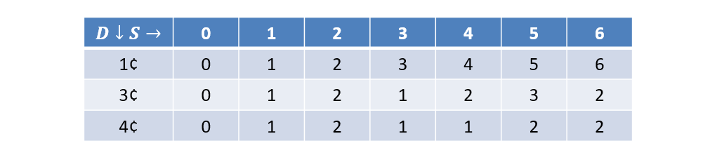
Now that we know the minimal number of coins in each cell, collecting the optimal solution is just a walk in the park... or rather, a walk through the table.

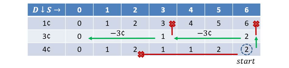
Starting at the bottom-right of the table:

If $T[r][c] == T[r-1][c]$, then the optimal solution came from denominations above, so recurse on $T[r-1][c]$.
Else, we used a coin from this denomination to get to $T[r][c]$, so collect that coin in our final solution then recurse on $T[r][c-D[r]]$.
Return full solution of collected coins when $T[r][c] == 0$.

This operation looks like the following in our running example, with the green up arrows indicating Case 1 above, and the green left arrows indicating Case 2:

Neat!

For a final consideration, if we have $R = |D|$ (number of denominations) and $C = S+1$, what is the asymptotic runtime / space complexity of these tabular methods?

Pretty simple: gotta compute each cell, so we have $O(R*C)$!

Top-Down DP

Compared to the part of the memoization structure that we *used* in finding the final answer using Bottom-Up DP on the Changemaker problem, what do we notice about the amount that we *completed?*

Many cells were completed unnecessarily!

It turns out this observation is indeed the motivating principle behind Top-Down Dynamic Programming.

Rather than starting at the simplest-subproblems-up, top-down starts with the biggest problem and recursively targets *which* subproblems it will need to solve in order to know the final answer.

The result will look similar to our search operation but is guided by the memoization structure to improve upon its asymptotic guarantees.

Reflect upon our recurrence for the Changemaking problem:

\begin{eqnarray} T[r][c] = \begin{cases} T[r-1][c], & \text{if}~D[r] \gt c \\ min(T[r-1][c], 1 + T[r][c-D[r]]), & \text{if}~D[r] \le c \end{cases} \end{eqnarray}

Let's observe how we can use this starting now at the bottom-right corner of the memoization structure:

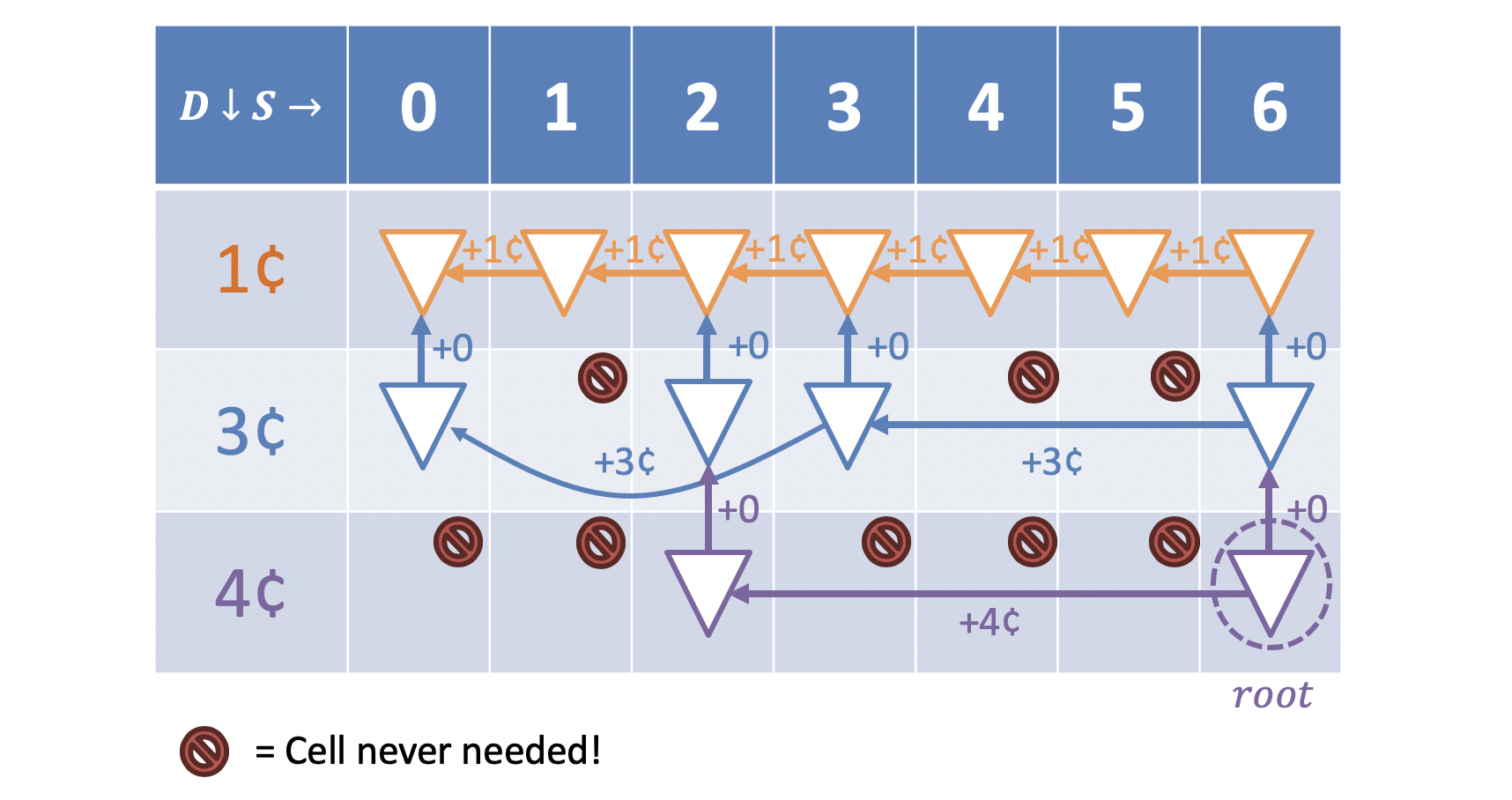
Filling in this structure would give us the following result:

Because Top-Down DP will still complete at most every table entry, its computational and space complexity are still bounded above by $O(R*C)$ for the given number of rows $R$ and columns $C$ in the table.

With the same asymptotic guarantees, when do we prefer one over the other?

Dynamic Programming - Strategy Juxtaposition

By now, we've seen both strategies to Dynamic programming: from the bottom-up and from the top-down.

Reasonably, you might have some follow-up questions related to now seeing both:

How are they similar? They seem to be very different approaches, albeit to the same types of problems. Is there any way to connect the dots between them?
How are they different? Practically, are there situations in which we'd like to use one over the other? What are their strengths and weaknesses?
Are they both only good for making change? Heck no! Post-Exam, we'll see another practical application of Dynamic Programming that's used in biology research, spellcheckers, and other domains all the time!

Similarities

There's too much strife in the world -- why start by focusing on the differences when we can focus on all of our common ground?

Compare our bottom-up and top-down solutions to the Changemaker problem with $D = \{1, 3, 4\}, S = 6$.

In the bottom-up approach, we complete the memoization table from top-left to bottom-right.

In the top-down approach, we perform what is essentially a "targeted-search-with-memoization" problem, in which we can depict the search / recursion tree starting at the root of the memoization structure (bottom-right corner) and then attempting to minimize the cost associated with the solution path:

So, seeing both, we can possibly intuit how they are similar; both certainly perform the same task (provide the optimal solution to the Changemaker problem specified), but there's an interesting similarity in how they go about this task.

The two are similar in that they both complete the necessary cells of the memoization structure to find the optimal solution by optimally solving sub-problems. It's *how* they complete the table that's different.

Differences

Alright, I think that about does it for intuition-building and comparison... let's get down to the brass tacks... the differences between these two approaches.

The primary difference between top-down and bottom-up DP: which, and how many, subproblems get solved: Top-down is selective, bottom-up is exhaustive.

How about we outline the implications of this difference? How about in a table? It's thematic because tabulation!

Criteria	Bottom-up DP	Top-down DP
Runtime - Many Overlapping Subproblems	Most of the memoization table will be relevant, in which case completing them iteratively leads to better wall-clock time with bottom-up due to iteration.	Although completing as-many or fewer cells of the memoization table, top-down will be slower in wall-clock time due to the rather costly nature of recursive calls.
Runtime - Few Overlapping Subproblems	Most of the memoization table will be irrelevant, in which case bottom-up wastes a lot of effort getting to the punchline.	Targeting only specific parts of the memoization structure improves efficiency if many cells remain unused, especially in larger problem.
Space	Fills whole table, solves all subproblems, taking up maximal space.	Fills only those table entries that are required, but the space is still reserved for the whole table.

tl;dr: Use bottom-up when lots of subproblems need to be solved, top-down when fewer.

Comparisons with Search

At face value, top-down DP looks a lot like how we formalized and then solved the changemaking problem with a search tree -- and in a lot of ways, they're the same!

The key differences:

Often, we cannot easily construct the memoization structure for a search problem, and so must rely on the search space's exploration via the tools of previous lectures.
Even if we can, sometimes it's just too dang large to realistically memoize using the structured table (since, even using top-down, memory is reserved in the table whether or not we're using that slot).
Using graph search to solve most top-down DP problems is a roughly equivalent technique, though can also be guided by heuristics in the case of A*.

tl;dr: use Dynamic Programming when you can structure the memoization and will need it for a *lot* of overlapping subproblems; use search when you can't, or the search can be guided to avoid much overlap.