Memory Allocation
Last time we examined some ways of viewing the logical memory addresses associated with a particular process' image, as well as how those addresses correspond to the programmer's perspective in source.
However, we should now consider how the logical / virtual addresses correspond to the physical ones in the RAM hardware itself.
Memory Allocation is the procedure of reserving physical memory addresses for processes.
Generally, allocation involves dividing physical memory into some number of partitions that will have allocation-strategy-specific interpretations.
By allocation-strategies, we mean that there are different ways to define the mapping between logical and physical memory, whose details and specifics will be the topic of today.
Depending on the approach, we should note: the logical memory image we consider when programming and the physical memory image in RAM may actually be quite different from strategy to strategy!
As such, let's start examining some strategies for providing this mapping.
Contiguous Allocation
What is the simplest way to partition RAM to provide a mapping between logical and physical addresses?
Have each logical memory image be dynamically mapped to an equivalently sized, contiguous partition in physical memory!
Contiguous Memory Allocation is an allocation strategy in which each process is contained within a single, contiguous section of physical memory.
In other words, if the logical address space of a process is 1000 addresses, we would expect it to mapped to some range of 1000 addresses in physical memory, like \([500, 1499]\) (in the case that the base of the partition was 500).
Because we know that this address binding is done at execution time in most operating systems, it is sometimes known as the variable-partition scheme.
In the variable-partition scheme to memory allocation, the OS keeps a table of the:
Partitions allocated to each process, including their addresses in physical memory and size.
Holes that form the free space (i.e., the addresses not in a partition), including their addresses and size.
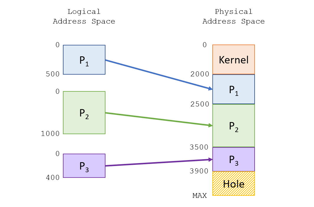
Take the following contiguous allocation with 3 processes, \(P_1, P_2, P_3\), and observe the mapping between their logical and physical addresses via contiguous allocation.
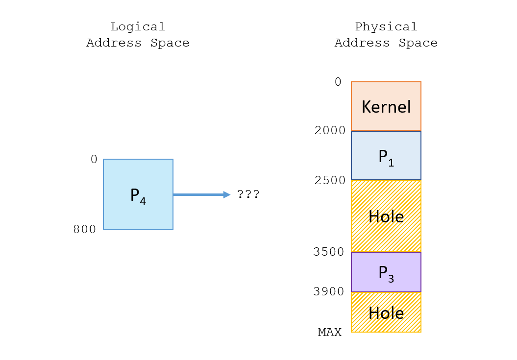
The beauty (and danger!) of dynamic storage is that processes come and go -- whenever a process has terminated, we are left with a hole in its place.
Continuing our example above, suppose \(P_2\) terminates and we are presented with a new process \(P_4\) in the input queue.
There are really three cases to consider for how we should allocate memory for a new process in the input queue:
How should we accommodate the front process in the input queue if there are NO holes large enough to fit it?
Either wait for other processes in RAM to terminate, or perform a swap if the scheduler demands it.
How should we accommodate the front process in the input queue if there is ONE holes large enough to fit it?
Allocate it within that hole, obvs...
How should we accommodate the front process in the input queue if there are multiple holes large enough to fit it?
We can choose one of them by some selection strategy.
Generally, when we are faced with multiple open holes big enough to accommodate a new process, we have a choice to make by some strategy.
The procedure for selecting which hole is chosen for a new process' allocation is known as the dynamic storage allocation problem, and is generally approached by one of three strategies.
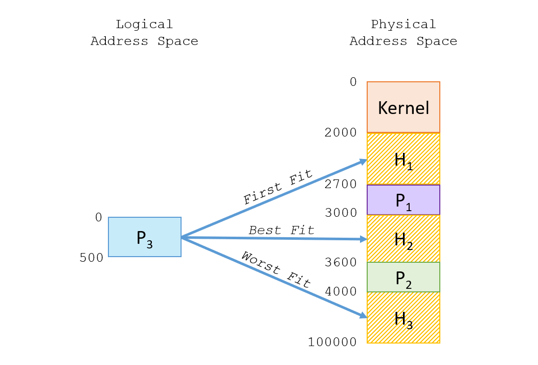
Suppose we have some processes \(P_1, P_2\) in RAM and are trying to fit \(P_3\) in one of a variety of holes with different characteristics; where should we place \(P_3\)?
These strategies were common in the early days of OS design and have a swath of empirical testing behind them and are formalized as:
First Fit allocates the process to the first available hole that is large enough. Benefit: fastest, but may not fit well.
Best Fit allocates the process to the smallest available hole that is still large enough to fit it. Benefit: leaves least space that may be wasted but must analyze all available holes.
Worst Fit allocates the process to the largest available hole that is still large enough to fit it. Benefit: leaves largest holes for others to use but must analyze all available holes.
Which strategies do you think performed the best, empirically, and why?
First fit (due to speed) and best fit (due to least wasted space), but in practice, best fit is too computationally expensive to use.
Still, the notion of wasted space is completely nontrivial; to use first fit means that we're willing to accept less-than-perfect fits in the name of performance.
As processes are loaded and removed from memory, free holes becoming uselessly small between allocated processes is known as external fragmentation.
External fragmentation squanders memory in the contiguous allocation schema because large process images cannot fit into the small holes, and it is too costly to relocate existing processes to remove them.
Approximately how much memory do you think is wasted due to external fragmentation if the First Fit approach is employed?
In empirical studies, the First Fit approach to the dynamic storage problem experiences an average loss of \(0.5N\) blocks of free space for each of \(N\) allocated blocks (the \(50\%\) Rule) -- so we end up wasting approximately \(\frac{1}{3}\) of RAM due to external fragmentation!
Due to the \(50\%\) Rule, we can start to see that contiguous allocation really breaks down... but perhaps there's another way to organize processes in memory...
If the problem with contiguous allocation is that we struggle to fit processes into fragmented free space, can you propose another approach that may serve as a solution?
Well uhh... how about we *don't* allocate contiguously? Let's chop up memory into smaller, bite-sized chunks!
Paging
Paging is another approach to partitioning wherein the physical addresses of a process are partitioned into smaller component pieces and need not be allocated contiguously.
Paging addresses the problem of external fragmentation and, to a large degree, the need to waste computation trying to find the "best" hole for a process' image.
The implementation details plainly require some hardware support, and are implemented differently accross architectures, but the general approach is the same:
Basic Paging Implementation
Paging implements a mapping between logical and physical memory through two fundamental components:
Frames are fixed-sized blocks of physical memory.
Pages are fixed-sized blocks of logical memory of the same size as each frame.
Loading a process into memory is thus done by copying pages into available frames.
So, how do we know who's who if we're scattering pages all over the place?
A page table provides a mapping between logical and physical addresses, and is typically stored per-process in RAM (often in Process Control Blocks).
Each logical address can thus be composed as a combination of:
Page number (p) used as an index in the page table to lookup its corresponding frame base address.
Page offset (d) combined with the base address to define the byte offset with the given page and corresponding frame.
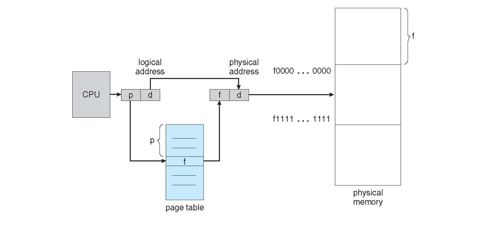
Pictorially, each address is a composite of:

The full translation process is depicted below:
For one last example, consider the following translation on a tiny 4-byte memory system to see how a page table can be maintained.
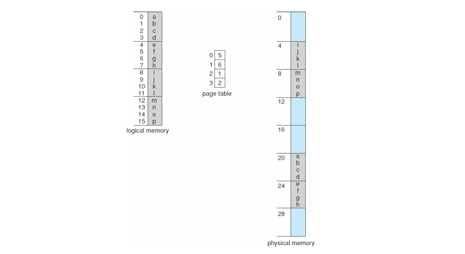
Observe, above, that the 'f' would have logical address 5 (page 1, offset 1)
What, then, is the physical address of 'f' translated using the page table?
Since page 1 is mapped to frame 6, and 'f' has a page offset of 1, the physical address would be \(25 = (4 \times 6 + 1)\)
Put a bookmark on this page, we'll return to it next time in a little greater detail!