Last time, we started to motivate what a "good" scheduler's metrics of success should be, and while the best approaches try to tick as many of these boxes as possible, there are certain tradeoffs that each approach makes, and we should be equipped to analyze these tradeoffs.

Before then, we need to formalize a few more details on what, precisely, we are trying to accomplish, and crystallize what is happening during a process' lifetime employing the CPU.

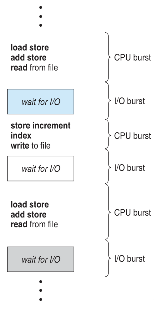
CPU Bursts

---

Pictorially, the cycle appears as (from your book):

Between I/O Bursts and CPU Bursts, which should the scheduler be most concerned about? Hint: consider that a scheduler must manage many processes.

CPU Bursts, since processes cannot typically proceed before their I/O Burst is completed, and therefore the scheduler must "fill the gaps" left in the CPU utilization whenever a process is waiting for an I/O event to complete.

While a scheduler is responsible for determining which process should be sent to the CPU for processing next, it is not the entity that dispatches it.

The dispatcher is the OS module that gives control of the CPU to the process next selected by the short-term scheduler.

It is the dispatcher that handles many of the important tasks associated with the swapping of processes currently using the CPU and those in the ready queue, including:

• Context switches (saving and restoring PCB states to then load into the CPU)

• Switching to user mode in dual-bit operation

• Setting the program counter to the proper location in the user program to restore its control flow

As we know, with any context switch comes some computational cost -- the dispatcher is a part of the interrupt process itself, and therefore incurs some overhead with every swap.

In general, we refer to this as dispatcher latency, the time it takes the dispatcher to swap out one process for another.

So how do we consider all of our optimization targets and dispatcher latency in design of a good scheduler? Let's look at some candidate approaches...

We already know that a scheduler is a module of an OS, and is itself a program with its own data structures and algorithms for determining which process should next be dispatched.

Formally, a scheduler maintains a schedule, which is a queue of processes and alloted burst quantums (time allotted for CPU use) that will determine their order of dispatch.

Given the metrics of scheduling success (maximizing throughput, CPU utilization, and minimizing turnaround, wait, and response time), what would be a basic way to "score" how well a scheduler is doing on these optimization criteria?

The average length of time that all processes are waiting in the ready queue, \(W_{avg}\)! This gives a good indication of throughput and the waiting times.

CPU utilization is somewhat harder to measure, because it is difficult to predict (in the abstract) which processes will require more I/O requests than others, which might otherwise play into scheduling concerns.

While there are other, more sophisticated, measures of comparison than average waiting time (see textbook), we'll discuss the latter herein.

Let's look at an example and start to consider some scheduling approaches:

First-come First-served (FCFS) Scheduling

---

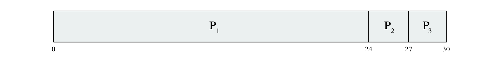
Suppose we have 3 processes \(P_1, P_2, P_3\) each with their own amount of time required for a single CPU burst (i.e., until they either transition to waiting for an I/O event or terminate, as detailed below); consider some scheduling approaches and the average time each would spend waiting.

Arrival Order	Process	Single CPU Burst Time (ms)
\(1\)	\(P_1\)	\(24\)
\(2\)	\(P_2\)	\(3\)
\(3\)	\(P_3\)	\(3\)

What is the most basic manner by which we could schedule these 3 processes?

The order in which they arrive!

This is certainly one of the simplest schedulers to implement and has a formal definition as:

A First-come First-serve (FCFS) approach schedules processes in the order in which they arrive, and allots them CPU bursts until completion (assuming no other interrupts).

To assess the merit of a scheduling approach, we can generate a Gantt Chart that depicts how long each process is waiting in the ready queue.

For the FCFS approach, the resulting Gantt chart looks like the following:

Using the above, how much time do each of \(P_1, P_2, P_3\) spend waiting to be dispatched? What is the average wait time?

Each process spends the following amount of time waiting (in ms): $$W_{P_1} = 0; W_{P_2} = 24; W_{P_3} = 27$$ As such, the average wait time (ms) is: $$W_{avg} = \frac{W_{P_1} + W_{P_2} + W_{P_3}}{3} = 17$$

We can start to see how this might be problematic...

What is the main issue with the FCFS approach, and what metric of scheduling success is compromised?

The Convoy Effect: shorter CPU burst processes are stuck behind longer ones, and so throughput is not maximized, and wait time is not minimized.

Suppose instead we had received the above processes in a different order:

Arrival Order	Process	Single CPU Burst Time (ms)
\(1\)	\(P_2\)	\(3\)
\(2\)	\(P_3\)	\(3\)
\(3\)	\(P_1\)	\(24\)

This would give us the Gantt Chart:

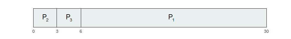
Using the above, how much time do each of \(P_1, P_2, P_3\) spend waiting to be dispatched? What is the average wait time?

Each process spends the following amount of time waiting (in ms): $$W_{P_1} = 6; W_{P_2} = 0; W_{P_3} = 3$$ As such, the average wait time (ms) is: $$W_{avg} = \frac{W_{P_1} + W_{P_2} + W_{P_3}}{3} = 3$$

Aha! So there's hope after all; we can see that just a small change in the order of scheduled processes can make a significant difference in the average wait time.

Suggest a scheduling algorithm that avoids the convoy effect.

Serve the shortest CPU burst processes first!

Shortest-Job-First (SJF) Scheduling

---

The shortest job first (SJF) scheduling algorithm associates with each process the duration of its next CPU burst, and then schedules them from least to greatest.

SJF is optimal, and will provably minimize the average wait time for processes.

We can see this in action and note that it does indeed minimize wait time; below, the order of arrival does not matter since we are ordering any processes remaining in the ready state based on their evaluated next burst time:

Process	Next CPU Burst Time (ms)
\(P_1\)	\(6\)
\(P_2\)	\(8\)
\(P_3\)	\(7\)
\(P_4\)	\(3\)

Thus generating the Gantt Chart:

...with an \(W_{avg} = (3 + 16 + 9 + 0) / 4 = 7\)

There's just one problem with SJF...

There's a major impediment to the implementation of SJF -- what is it?

It is not possible for a scheduler to perfectly predict a process' next burst time!

That certainly puts a bit of a wrench in the gears for this approach!

However, all hope is not lost; we can try to get some semblance of a handle on these next burst times.

Without knowing each process' exact duration for its next CPU burst, how could we use SJF scheduling?

Make a prediction about the next burst time based on the previous ones!

This makes some intuitive sense: we would expect that a process takes CPU bursts that last more or less the same amount of time, and that we can use its history to predict the future.

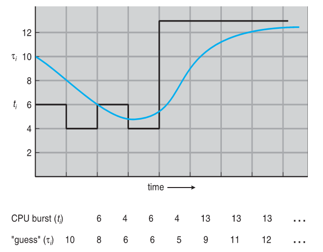
Although you do not need to know the following intimately for this class, you should be aware that this prediction step can be well approximated using exponential averaging, defined by:

This predictive "smoothing" yields the ability to quickly, and sufficiently accurately predict future burst times of processes without much burst variance, as can be seen in the example graph below:

Priority Scheduling

---

With the wait-minimizing capacities of SJF, we should consider:

What are some reasons, other than minimizing wait time, that we may want to give a process early acces to the CPU?

OS-critical processes, time limits, memory requirements, ratio of I/O to CPU bursts, etc.

In these cases, we have priorities that may not necessarily be the processes with the shortest CPU burst.

Instead, we can schedule processes based on a given score, i.e., its priority.

Priority Scheduling associates a priority score with each process, and then dispatches those with the highest priority first.

Process	Next CPU Burst Time (ms)	Priority (Lower Score = Higher Priority)
\(P_1\)	\(10\)	\(3\)
\(P_2\)	\(1\)	\(1\)
\(P_3\)	\(2\)	\(4\)
\(P_4\)	\(1\)	\(5\)
\(P_5\)	\(5\)	\(2\)

Thus generating the Gantt Chart:

Note: SJF is simply a special case of the general priority scheduling in which priority is the inverse of estimated next burst time.

Thus, priority scheduling gives us more power to customize what factors should contribute to a process' importance, and the flexibility to include wait time as part of that scoring process.

However, priority scheduling is vulnerable to one important pitfall:

Suppose a process with a low priority is waiting to be run, and many high priority processes jump ahead of it in line; what could happen in the most detrimental case?

Starvation: a process may never be dispatched if new, higher priority processes keep jumping in front!

Propose a solution to starvation in priority scheduling.

Aging: heighten the priority of a process the longer it has been waiting!

Round-Robin Scheduling

---

Lastly, developed for time sharing systems but used in a variety of contexts, we may have systems in which many users are attempting to employ the CPU at once, and it would be unfair to prefer one user over the other.

Round-robin (RR) scheduling sets a maximum time quantum \((q)\) (slice of time alloted to each process) that a dispatched process has to execute, and if it is not terminated within that quantum, is placed back at the end of a circular queue.

In other words, using Round Robin scheduling, no process employs the CPU for more than 2 consecutive "turns" unless it is the only ready process.

Returning to our initial example, and choosing a time quantum \(q = 4\):

Arrival Order	Process	Single CPU Burst Time (ms)
\(1\)	\(P_1\)	\(24\)
\(2\)	\(P_2\)	\(3\)
\(3\)	\(P_3\)	\(3\)

And thus...

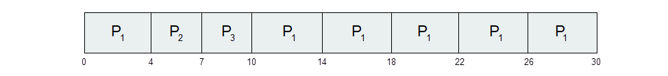
Thus gives us an average waiting time of: $$W_{avg} = \frac{W_{P_1} + W_{P_2} + W_{P_3}}{3} = \frac{(10-4) + 4 + 7}{3} \approx 5.66$$

RR, apart from its benefits to fairness, typically boasts a higher average turnaround time compared to SJF, but has better response.

The only foible with RR is one's choice of quantum time, since a quantum that is too large can hinder response times, but a quantum that is too small will incur overhead from context switches:

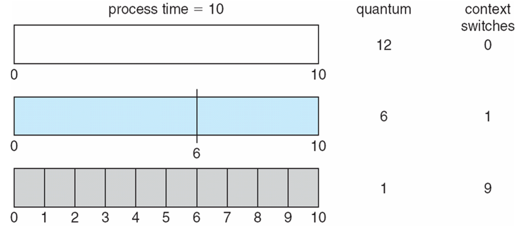
Choices for quantums are generally between 10 - 100 ms, but vary between OS' that employ the RR technique.

Which brings us to our final topic... what schedulers are modern OS' using?

So how are modern OS' scheduling?

OS	Scheduling Approach
Windows	Priority-based with preemption 32 priority levels split between variable and real-time classes
Mac OS X	Policy-based with preemption, but priority is embedded into assigned policy Different policies apply different constraints on priority, e.g., the standard policy is a fair sharing alg., and a time constraint policy balances real-time needs.
Linux	Priority-based with preemption 141 priority levels split into real-time (0-99) and nice (100-140) where nice scores can be set by user to modify real-time priority. Higher the priority = higher the time quantum

To say a little more about the Linux approach, the priorities are actually stored in a balanced Red-Black Tree to compose its "completely fair scheduler (CFS)"

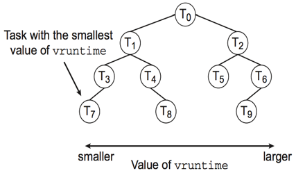
The CFS red-black tree stores the time that each process has had with the processor in each node, and uses this as a part of its priority.

The CFS scheduler proceeds as follows:

1. Left most leaf is chosen for execution (highest priority, lowest time spent executing).

2. If it terminates, it is removed from the tree and tree is rebalanced.

3. If the time quantum is exceeded, the node's execution time is updated, and resorted into the tree.

4. Repeat.

This is considered fair because it marries the RR approach of time quantums with the ability to customize priorities as seen fit.

You can check active process' priorities using the ps -el command in bash -- give it a shot!