Improving Backtracking

Recall our numerical CSP with 3 variables from last lecture, and observe some opportunities to improve upon how the backtracking played out (including ways to prevent unnecessary work from the start)!

[Reflect] What are some wasteful elements or possibilities for computational improvements of backtracking applied to the CSP as specified above?

To name a few:

Some variable domains are too loose:
- Consider constraint #2: in order to satisfy this constraint, we know that $R \ne 2$.
- Consider constraint #3: in order to satisfy this constraint, we know that $T \ne 0$ and $S \ne 2$, so keeping these values in their domain leads to waste in the backtracking.
The order in which we chose to assign values to variables and the order in which we choose variables to assign to can matter!

These observations lead to two common improvements to backtracking that can have a profound impact on the capacity of CSP solvers to derive solutions to nontrivially sized CSPs in a tractable amount of time.

We'll look at these next!

Filtering

From our reflections above, we noted that, even at the start, there are certain values in variable domains that, due to certain constraints, will *never* be part of a solution.

[Brainstorm] How could we save ourselves some work from this observation?

Reduce these domains to only plausible values before backtracking begins!

Filtering is a technique for improving backtracking wherein the domains of unsassigned variables are then reduced by examining constraints and assignments to other variables.

Filtering helps us to reduce the branching factor of the recursion tree during backtracking, making some large CSPs solvable in a reasonable amount of time!

There are various ways that we can filter "bad values" from domains, ranging from the simple to more forward-planning.

Let's consider how to go about this "pruning" process.

Constraint Graphs and Consistency

Earlier, when dealing with the Map Coloring problem, we created a graph of the adjacent nation-states:

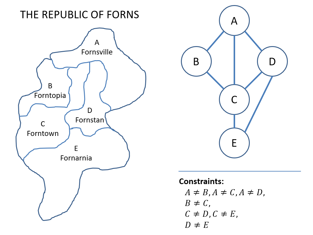
Why might similar graphs be useful to create in other CSPs as well?

We can use them to determine what variables' domains are dependent based on which are found in the same constraints!

Constraint Graphs are structures of CSPs useful in filtering such that:

Nodes are variables.
Edges connect any two variables that appear in a constraint together.

Using these graphs, we can then verify that, at any stage, the values in each variable's domains are those that are still *useful* to consider.

Variable domains are said to be consistent when they contain only values that are potential candidates for a solution.

We can therefore check for various granularities of consistency as aided by these constraint graphs.

Starting with the simplest kind of consistency check:

Node Consistency is a filtering technique that ensures domains are consistent for any unary constraints pertaining to a particular node / variable in the constraint graph.

Here, "unary constraint" means a constraint that involves only a single variable.

Examine the simple CSP with two variables possessing different domains:

\begin{eqnarray} X &=& \{A, B\} \\ D_A &=& \{0, 1, 2\} \\ D_B &=& \{0, 1, 2\} \\ C &=& \{ \\ &\quad& B \lt 1, \\ &\quad& A \ne B \\ \} \end{eqnarray}

In this example, it's fairly obvious that the first constraint is unary and restricts the domain of $B$.

The repair is likewise simple: remove the values from $D_B$ that can never be a part of a solution.

Enforcing Node Consistency for node $B$:

$$D_B \leftarrow \{0\}$$

Node $A$ is already node consistent (there are no unary constraints on $A$):

$$D_A \leftarrow \{0, 1, 2\}$$

With this updated domain, we'll end up saving ourselves a lot of work (well, maybe not for this example, but in general!)

Yet, examining the *new* domains after enforcing node consistency, do we detect any other opportunities to ensure consistency?.

Yes! Note that since $B$ can only be $0$, and since $A \ne B$, $A$ *cannot* be $0$, and so this should be removed from its domain.

This deduction was possible because we knew that $A, B$ were connected in certain constraints, and therefore adjacent in the constraint graph.

As such, to check consistency *between* variables, we perform a new type of check:

Arc Consistency is a filtering technique that ensures domains are consistent for any binary constraints pertaining to any pairs of adjacent nodes in the constraint graph.

Reasonably, you might observe that this is called arc, rather than edge, consistency -- why is this the case?

Using a constraint graph in which two adjacent variables $A, B$ are connected by an edge:

Consider two directed edges between $A, B$ with one variable at the "tail" and another at the "head" such that $tail \rightarrow head$: $(A \rightarrow B), (B \rightarrow A)$.
A directed arc is consistent if and only if for all values in the tail domain there is at least one value in the head domain that satisfies the arc's constraint.
Values in the tail with no satisfying values in the head are removed from the tail domain.

Depicting how we "unpack" the arcs in our simple example above, we have:

Intuitively, in our example above, we see how the domain of $A$ gets restricted due to arc consistency:

Recapping: \begin{eqnarray} D_A &=& \{0, 1, 2\} \\ D_B &=& \{0\} \end{eqnarray}

Enforcing Arc Consistency $B \rightarrow A$:

There is at least one value in $D_A$ that satisfies the only one in $D_B$ (namely, if $B=0$, then $A=1$ satisfies the arc's constraint). So, we need not modify $D_B$.

Enforcing Arc Consistency $A \rightarrow B$:

There is no value in $D_B$ that satisfies the arc constraint for $A = 0$, therefore, we prune it from the domain of $A$:

$$D_A \leftarrow \{1, 2\}$$

Neat! So we see that through enforcing node and arc consistency, we reduce the domains of variables to make backtracking easier.

We should note that checking for arc consistency does *not* perform the backtracking itself; consider the following tweaked example from above:

Suppose we have an even simpler CSP: \begin{eqnarray} X &=& \{A, B\} \\ D_A &=& \{0, 1\} \\ D_B &=& \{0, 1\} \\ C &=& \{ \\ &\quad& A \ne B \\ \} \end{eqnarray}

Are $A, B$ arc consistent in the above?

Sure! Each has at least 1 value in the other domain that can satisfy each of its values for the constraint $A \ne B$.

So, taking a step back, we should note that using Filtering, we end up with one of several outcomes:

Filtering reduces a domain to the empty set: Easy! No solution to this CSP.
Filtering reduces each domain to a single value: Easy! Don't need to even backtrack, we have our solution.
Filtering reduces each domain to some multitude of values: Still requires backtracking to find a solution.

As such, Filtering can be used as both a preprocessing tool to reduce work before backtracking, as well as a tool for filtering as values are assigned during backtracking.

Forward Checking

Forward Checking is a filtering technique deployed during backtracking that removes values from domains via arc-consistency when values are added to an existing assignment.

In other words, during backtracking, suppose we assign a value to a variable in one of the partial states. Using forward checking this then restricts the domains of variables that are yet to be assigned by the tenets of arc consistency.

Consider a simplified Map Coloring problem with $K = 3$ colors in which, during backtracking search, we assign: $$B = Blu, D = Red$$

Above, we would appropriately restrict the domains of $A, C$ to the last remaining color by the tenets of arc consistency.

What's the problem with these restricted domains?

Forward checking did not detect an early failure that would result from its assignments since it is not possible for both $A, C$ to share the same color, despite the correct reductions to their domains.

Any suggestions for how to give some chance at catching these inevitable failures sooner?

Propagate restrictions between constraints rather than just between nodes!

Put differently, let's attempt to take any domain restrictions we make, and then propogate those changes through the other arcs as well!

Constraint Propagation

Constraint Propogation is a filtering technique in which any changes to domains made by arc consistency are propogated to neighbors in the constraint graph.

The general idea: each time a change to a domain is made by arc-consistency, re-check the neighbors of the modified domain in the constraint graph. Repeat this process until all arcs have been made consistent.

The AC-3 (arc-consistency, 3rd edition) Algorithm can be used to proceduralize constraint propagation.

In gist, the steps of AC-3 are:

Maintain a Queue of arcs $(tail, head)$ to check for consistency, starting with *all* arcs in the Queue.
While the Queue is not empty, pop an arc:
1. If it's consistent, continue!
2. If it's inconsistent, remove the offending values from the tail domain, then re-add all neighboring arcs that point to the tail (i.e., all adjacent nodes that point to the tail that are also *not* the head) back into the Queue.

Or, more formally, the algorithm is stated as:

Return to our 3-variable example with $R, S, T$ and trace the execution of AC-3 on it to reduce the variable domains!

\begin{eqnarray} X &=& \{R, S, T\} \\ D_i &=& \{0, 1, 2\}~\forall~X_i \in X \\ C &=& \{ \\ &\quad& R \ne S, \\ &\quad& R = floor(T / 2), \\ &\quad& S \lt T \\ \} \end{eqnarray}

Let's start by being clear about the arcs in our constraint graph:

Now, with our initialization for AC-3...

...we trace the steps of AC-3!

Note: in the above example, the queue additions ended up not being significant, but they might be in general! The above was merely meant to show you the steps and mechanics of AC-3.

Whew! That might've felt like a lot of steps, but the savings are tangible -- we trimmed a value off of each domain, which (for large problems) can have a profound performance effect.