Last lecture we started to see some of the shortcomings in Bayesian Networks (BNs) to answer more nuanced queries of a causal nature.

Instead, we need some stronger causal assumptions about the system in order to answer these interesting queries.

As such, today we take our first steps towards the next wrung in the causal hierarchy -- look at that little fellow climb!

When we want to formally state our causal assumptions about a system of variables, we need a formal language to express the following:

1. What variables are causal influences on what other variables.

2. What variables are relevant, but are perhaps unable to be measured or are unknown entirely.

3. What is the nature of the effect that some cause has on another.

4. How to encode chance, probability, and statistics from missing, unobserved, or latent causes.

In the future, we'll look at how to model these pesky unobserved variables, and what the implications are for our models.

For now, let's worry about modeling the observed variables using a flexible framework known as a Structural Causal Model, defined as follows:

A Structural Causal Model (SCM) specifies the modeler's assumptions about a system of cause-effect relationships, and is formalized as a 4-tuple \(M = \langle V, U, F, P(u) \rangle \) consisting of the following components:

I. \(U\), Exogenous Variables: a set of observed variables \(U = \{U_0, U_1, ..., U_u\}\) whose causes are unknown or not included in the model.

You can remember these as variables whose states are decided by factors outside of, i.e., external to, the SCM, even though these factors likely exist in the true model of reality, which we are merely sampling.

Give some examples of exogenous variables! Here are a couple: eye color (influenced by unobserved genetics) and states of an atom (affected by unobserved quantum mechanics).

II. \(V\), Endogenous Variables: a set of observable variables \(V = \{V_0, V_1, ..., V_i\}\) whose causes are known and included in the model -- either as exogenous or other endogenous variables.

Endogenous variables are those that we are claiming to have the "full picture" on.

Give some examples of endogenous variables! Here's one: the salary of an employee if you modeled two exogenous causes: starting salary, duration at company, and scheduled raises.

III. \(P(u)\), Probability Distributions Over All \(u \in U\): because exogenous variables' causes are unobserved, we can only speculate about their state through some probability distribution assigned to each. Additionally, since all endogenous variables have at least 1 exogenous ancestor, \(P(u)\) elicits a probability distribution over \(P(v)~\forall~v \in V\).

This facet of a SCM can feel a bit unintuitive, so let's consider an example to make things a bit more concrete.

Consider a simple study in which we have collected data on a population's Eye Color [E].

If Eye Color is an exogenous variable in the system, what might be an unobserved cause of \(E\)? Something we might even be aware of but would find difficult to measure?

An individual's genetics!

Depicted below, we can see that there is some mapping of the latent probability space (which can have some enormous number of states that we will not see), to the exogenous space, which has some number of states that we *can* measure.

Important notes for the above:

• We may know the distribution over \(G\) above, even if we're not easily able to condition on its state for the arbitrary individual!

• If we *did* know the state of every exogenous variable, we could determine the state of any \(V\) in the model with perfect accuracy (in theory, at least!), even though we must represent the exogenous causes probabilistically.

IV. \(F\), Structural Equations: a set of functions \(F = \{f_{V_0}, f_{V_1}, ..., f_{V_i}\}\) for each endogenous variable that describes how each variable responds to its observed causes.

Note: these functions can describe any relationship and are not limited to probabilistic expressions.

They are called "structural" because they are meant to uncover / model the "structure" of causes and effects in the system, and exhibit some nice, causal properties that we'll see in a moment.

The vocabulary of "cause" is thus dictated by these structural equations: if a variable \(X\) appears as a parameter to another's \((Y)\) structural equation, then we say that \(X\) is a direct cause of \(Y\).

Take, for example, structural equations defining a system of Years of Higher Education \(E\), Years of Work Experience \(W\), and Salary \(S\). We have: $$SCM~ M_1:~ U=\{E, W\},~V=\{S\},~F=\{f_S\},~P(u)=\{...\}$$ $$S \leftarrow f_S(E, W) = 12,000*E + 5,000*W$$

If we were *given* that someone had spent 4 years in higher education, 3 years in the workforce what would we expect for that individual's salary?

We would expect \(S = f_S(4, 3) = 12,000*4 + 5,000*3 = 63,000 \) (the exact mathematics and notation of which we'll cover later when we look at a particular type of SCM for linear modeling).

OK! Nothing too complicated; looks like SCMs are just flexible models that can represent cause-effect relationships using functional notation.

But...

What seems to be the major difficulty with SCMs?

Knowing the *true* \(F\) for the system in reality!

Can you think of some scenarios wherein we *may* know the true structural equations?

Modeling logical problems, rules in video games (wherein the programmers are "god"), known laws of physics, etc.

In a nutshell: having the exact structural equations is nice and allows for powerful prediction, but when we lack them, we can instead try to estimate them in a model that can still answer queries within statistical tolerance.

This does not mean that lacking structural equations sinks us; there is still merit in knowing which variables we would like to model as causes of which other variables, even if we do not know precisely *how* they affect one another.

A partially-specified SCM is one in which we specify only what variables should appear as inputs in each structural equations, but do not know the exact equation itself.

So, if we did not want to commit to the structural equations in our Salary predictor above, we might leave it as a partially specified model such as: \begin{eqnarray} F &=& \{S\} \\ S &\leftarrow& f_S(E, W) \end{eqnarray}

Partially-specified SCMs serve as a "lens" through which we can interpret data, or to measure the relationships statistically.

To do so, we can also represent SCMs in a more intuitive format.

Graphical Models

---

Sometimes intuitions about SCMs can get lost in the structural equations, so we typically conceive of them using graphical notation, in a syntax that will look very familiar from our work with BNs.

This last bullet may be a bit surprising, but we'll see that d-separation is meaningful and useful in a variety of contexts and for a variety of different structural equation formats.

Even if graphical models provide less information than the fully-specified SCMs, they can lead to better intuition about the system, and expose interesting independence relationships through d-sep.

Modeling our Salary predictor example, graphically, we would have:

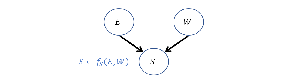
Hey, that looks an awful lot like a structure we're all familiar with! It looks like the structure of a BN, which is not incidental.

It turns out that one of the earliest SCMs was one that admitted to not knowing the structural equations, but can still be considered to carry causal information.

Let's look at it now!

Causal Bayesian Networks (CBNs)

---

A Causal Bayesian Network (CBN) is a type of partially-specified SCM wherein the structural equations \(F\) and distributions over exogenous variables \(P(u)\) are rolled into probabilistic distributions represented by traditional BN Conditional Probability Tables (CPTs).

Note that the only change between a BN and a CBN is that for a CBN, we are claiming that the structure indicates the correct direction of edges from causes to effects (i.e., there are no observationally equivalent models that should be considered apart from the one we're defending).

In brief: any time we conclude that our BN is causal (a CBN), we must be able to do so on sound, scientific, and defendable grounds.

Some relationships are easier to defend than others.

For example, suppose we add "Age" [A] as a variable to our heart-disease BN and found it to be dependent on variables \(V, E\). How would our network structure change and why is there only one interpretation for it?

Returning to our Vaping example, for now, let's suppose we're happy with our original BN and are able to (for now, hand-wavingly) defend it as a CBN. Can we answer our causal query yet?

Recall our causal query: "Does vaping cause heart disease?"

Suppose the structure of our CBN is now correct, we still have a problem with the Bayesian conditioning operation for examining the difference in conditional probabilities.

To remind us of this problem:

[Reflect] How can we isolate the effect of \(V \rightarrow H\) using just the parameters in our CBN?

I dunno... how about we just chuck the "backdoor" path?

More or less, yeah! That's what we're going to do through what's called an...

Intervention

---

I know what you're thinking... and for any Always Sunny fans out there, I have to reference with:

In our context, however...

An intervention is defined as the act of forcing a variable to attain some value, as though through external force; it represents a hypothetical and modular surgery to the system of causes-and-effects.

As such, here's another way of thinking about causal queries:

Intuition 1: Causal queries can be thought of as "What if?" questions, wherein we measure the effect of forcing some variable to attain some value apart from the normal / natural causes that would otherwise decide it.

With this intuition, we can rephrase our question of "Does vaping cause heart disease" as "What if we forced someone to vape? Would that change our belief about their likelihood of having heart disease?"

Obviously, forcing someone to vape is unethical, but it guides how we will approach causal queries, as motivated by the second piece of intuition:

Intuition 2: Because we're asking causal queries in a CBN, wherein edges encode cause-effect relationships, the idea of "forcing" a variable to attain some value modularly effects only the variable being forced, and should not affect any other cause-effect relationships.

So, let's consider how we can start to formalize the notion of these so called interventions.

If an intervention forces a variable to attain some value *apart from its normal causal influences,* what effect would an intervention have on the network's structure?

Since any normal / natural causal influences have no effect on an intervened variable, and we do not wish for information to flow from the intervened variable to any of its causes, we can sever any inbound edges to the intervened-upon variable!

Let's formalize these intuitions... or dare I say... in-do-itions (that'll be funny in a second).

The \(do\) Operator

---

Because observing evidence is different from intervening on some variable, we use the notation \(do(X = x)\) to indicate that a variable \(X\) has been forced to some value \(X = x\) apart from its normal causes.

Heh... do.

To add to that vocabulary, for artificial agents, an observed decision is sometimes called an "action" and a hypothesized intervention an "act".

"HEY! That's the name of your lab! The ACT Lab!" you might remark... and now you're in on the joke.

Structurally, the effect of an intervention \(do(X = x)\) creates a "mutilated" subgraph denoted \(G_{X=x}\) (abbreviated \(G_x\)), which consists of the structure in the original network \(G\) with all inbound edges to \(X\) removed.

So, returning to our motivating example, an intervention on the Vaping variable would look like the following, structurally:

[Reflect] How do you think this relates to how humans hypothesize, or ask questions of "What if?" Do you ignore causes of a hypothetical and focus only on its outcomes?

This will be an important question later, since intelligent agents may need to predict the outcomes of their actions.

OK, so we've got this mutilated (and yes, that's the formal, gory adjective) subgraph, which seems to represent the intervention's structural effect, but how does an intervention affect the semantics?

To answer that question, we can use Intuition #2 from above, considering that the intervention is modular, and should not tamper with any of the other causal relationships.

Because of this modularity, performing inference in the intervened graph \({G_{V}}\) equates to determining which parameters (i.e., CPTs) from the un-intervened system represented in \(G\) are the same.

If all latent variables are independent, or are not common causes of any variables, the SCM is called a Markovian Model, and all CPTs between the pre- and post-intervention will be the same except for the intervened.

This is because, for some intervention on variable \(do(X = x)\):

• The only structural equation modified by the intervention is \(f_X = x\).

• All structural equations that are not descendants of \(X\) will remain unaffected.

• All structural equations that are descendants of \(X\) already encode their behavior for different values of \(X\).

We'll see why this nice property holds for Markovian models next time, when we remove that restriction and see a more general class of SCMs.

That said, the modularity of a Markovian SCM establishes the following equivalences, if we denote the CPTs in the intervened graph as \(P_{G_{V}}(...)\):

\begin{eqnarray} P(S) &=& P_{G_{V}}(S) \\ P(E | S) &=& P_{G_{V}}(E | S) \\ P(H | do(V = v), E) &=& P_{G_{V}}(H | V = v, E) = P(H | V = v, E) \end{eqnarray}

The only asymmetry is that by forcing \(do(V = v)\), we replace the CPT for \(V\) and instead have \(P_{G_{V}}(V = v) = 1\).

Consider the Markovian Factorization of the original network (repeated below); how would this be effected by an intervention \(do(V = v)\)? $$P(S, V, E, H) = P(S)P(V|S)P(E|S)P(H|V,E) = \text{MF in Original Graph}$$ $$P(S, E, H | do(V = v)) = P_{G_{V}}(S, E, H) = \text{???} = \text{MF in Interventional Subgraph}$$

Since we are forcing \(do(V = v)\) (i.e., \(V = v\) with certainty apart from its usual causes), this is equivalent to removing the CPT for \(V\) since \(P(V = v | do(V = v)) = 1\). As such, we have: $$P(S, E, H | do(V = v)) = P_{G_{V}}(S, E, H) = P(S)P(E|S)P(H|V=v,E)$$

This motivating example is but a special case of the more general rule for the semantic effect of interventions:

Semantically, the effect of an intervention \(do(X = x)\) in a SCM is to replace the structural equation of \(X\) with the constant \(x\), i.e., $$do(X = x) \Rightarrow X \leftarrow f_X = x$$

In a Markovian CBN, this semantic effect of an intervention leads to what is known as the Truncated Product Formula, which is the Markovian Factorization with all CPTs except the intervened-upon variable's, or formally: $$P(V_0, V_1, ... | do(X = x)) = \Pi_{V_i \in V \setminus X} P(V_i | PA(V_i))$$

Example

---

You knew this was coming, but dreaded another computation from the review -- I empathize, this is why we have computers.

That said, it's nice to see the mechanics of causal inference in action, so let's do so now.

Using the heart-disease BN as a CBN, compute the likelihood of acquiring heart disease *if* an individual started vaping, i.e.: $$P(H = 1 | do(V = 1))$$

As it turns out, the steps for enumeration inference are the same, with the only differences being in the Markovian Factorization.

Hmm, well, doesn't seem like a huge difference, does it -- a mere ~1.5% is all we have to show for our pains?

Although it may not seem like a lot, keep the following in mind:

1. This is a small network, and therefore, little chance for things to go completely haywire. In larger systems with different parameterizations, these query outcomes can be much more dramatically different.

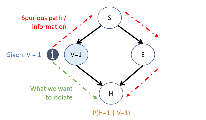
2. Note also the difference in information passed through spurious paths in the network based on the associational vs. causal queries (depicted below).

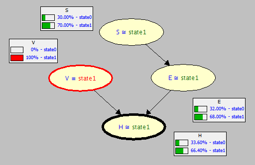
Note the CPTs for each node updated for observing \(V = 1\) in the original graph \(G\).

Sorry for the quality -- if you want to play around, this is a small Java app called SamIAm from UCLA -- it's a bit dated but gets the job done.

Now, note the CPTs for each node updated (or lack thereof) for intervening on \(do(V = 1)\) in the mutilated subgraph \(G_{V=1}\).

Conceptual Miscellany

---

How about a few brain ticklers to test our theoretical understanding of interventions?

Q1: Using the heart disease example above, and without performing any inference, would the following equivalence hold? Why or why not? $$P(H = 1 | do(V = 1), S = 1) \stackrel{?}{=} P(H = 1 | V = 1, S = 1)$$

Yes! This is because, by conditioning on \(S = 1\), we would block the spurious path highlighted above by the rules of d-separation. As such, these expressions would be equivalent. This relationship is significant and will be explored more a bit later.

Q2: would it make sense to have a \(do\)-expression as a query? i.e., on the left hand side of the conditioning bar of a probabilistic expression?

No! The do-operator encodes our "What if" and is treated as a special kind of evidence wherein we force the intervened variable to some value; as this is assumed to be done with certainty, there would be no ambiguity for it as a query, and therefore this would be vacuous to write.

Q3: could we hypothesize multiple interventions on some model? What would that look like if so?

Sure! Simply remove all inbound edges to each of the intervened variables, and then apply the truncated product rule to remove each of the intervened variables' CPTs from the product!

And there you have it! Our first steps into Tier 2 of the Causal Hierarchy.

But wait! We didn't *really* answer our original query: "What is the *causal effect* of vaping on heart disease?"

To answer the question of what effect Vaping has on Heart Disease, we can consider a mock experiment wherein we forced 1/2 the population to smoke and the other 1/2 to abstain from smoking, and then examined the difference in heart disease incidence between these two groups!

Sounds ethical to me! </s> </dangling-tags>

We'll talk more about sources of data and the plausible estimation of certain queries of interest in the next class.

That said, this causal query has a particular format...

Average Causal Effects

---

The Average Causal Effect of some intervention \(do(X = x)\) on some set of query variables \(Y\) is the difference in interventional queries: $$ACE = P(Y|do(X = x)) - P(Y|do(X = x'))~x,x' \in X$$

So, to compute the ACE of Vaping on Heart disease (assuming that the CBN we had modeled above is correct), we can compute the likelihood of attaining heart disease from forcing the population to Vape, vs. their likelihood if we force them to abstain: $$P(H=1|do(V=1)) - P(H=1|do(V=0)) = 0.664 - 0.164 = 0.500$$

Wow! Turns out the ACE of vaping is a \(+50\%\) increase in the chance of attaining heart disease!

Risk Difference

---

It turns out our original, mistaken attempt to measure the ACE using the Bayesian conditioning operation was not causal, but still pertains to a metric of interest in epidemiology:

The Risk Difference (RD) is used to compute the risk of those already known / observed to meet some evidenced criteria \(X = x\) on some set of query variables \(Y\), and is the difference of associational queries: $$RD = P(Y|X = x) - P(Y|X = x')~x,x' \in X$$

Computing the RD of those who are known to Vape on Heart Disease, we can compute the risks associated with those who Vape vs. those who do not: $$P(H=1|V=1) - P(H=1|V=0) = 0.649 - 0.182 = 0.467$$

Again, although the difference between the ACE and RD is only ~3%, this distinction can be compounded in larger models, and answers a very different, associational question than does its causal counterpart, the ACE.

All of today's (lengthy!) lesson seems to hinge on our models being correct, and as we'll see, on the data supporting them. Next time, we'll think about how we might still be able to answer queries of interest even if there are some quirks in either. Stay tuned!