Reinforcement Learning
We're trying things a bit differently this semester: I'm going to start with reinforcement learning and *then* talk about causal inference... let's see if my switcheroo is... reinforced or not!
We'll start, as always, with some background, motivating examples, and definitions, then look at formalisms for techniques in all of the above.
Distinguishing Reinforcement Learning
Reinforcement Learning (RL) describes a class of problems (and their associated solutions) in which an agent must map situations to optimal actions, but the best actions in any situation must be learned.
Examples of this sentiment are that RL agents may need to learn:
The best ad to show to a user of some demographic group.
The best move to make in a particular spot on a particular level of Super Mario Bros.
The best route to recommend to a driver during different times of the day.
Note that in all of these scenarios, the agent is often faced with the task of self-discovery: there may not be clear examples of the expected behavior, nor any human-provided guidance.
Sometimes, as is true of human learning, the best techniques are those of trial and error!
Moreover, we should be sensitive to how these types of problems and their approaches deviate from traditional data-centric machine learning...
[Review] What are supervised and unsupervised learning and how are their problems / solutions different from the above?
Supervised learning attempts to learn some function that maps features to some class label (i.e., learn the \(f\) in \(f(X) = Y\)) through a training set of existing data.
Unsupervised learning attempts to find structure / meaning in unlabeled data.
Reinforcement Learning differs from these in several chief regards:
Reinforcement learners may need to gather said data, rather than begin with it.
Reinforcement learners may wish to optimize behaviors that are not found in any example dataset (e.g., to play a game at superhuman levels, perhaps the best strategy cannot be learned from human-created data!)
Reinforcement learners may be *aided* by finding structure in the collected data, but operate chiefly by attempting to maximize some reward.
As we will see much later this semester, the best reinforcement learners may involve supervised and unsupervised components, but their chief focus is in maximizing some reward!
We can also juxtapose RL with Causal Inference and note that:
While Causal Inference seeks to *deeply understand and model* an environment, Reinforcement Learners primarily wish to *excel* in it (whether or not they've really understood it).
Despite these seemingly disparate goals, there are times wherein RL may aid CI and vice versa, as we shall see very shortly!
For now, let's be pedantic and detail the key components of reinforcement learning.
Properties of Reinforcement Learning
A hallmark of reinforcement learning is that an agent interacts with its environment in a feedback loop of agent action and environment reaction as the agent learns the best actions over time.
These terms apply liberally; an agent can be any intelligent system from a physical robot to an online ad selector, and the environment can likewise be flexibly defined as anything from the terrain on Mars to the sidebar on a webpage.
Pictorially (from your textbook):
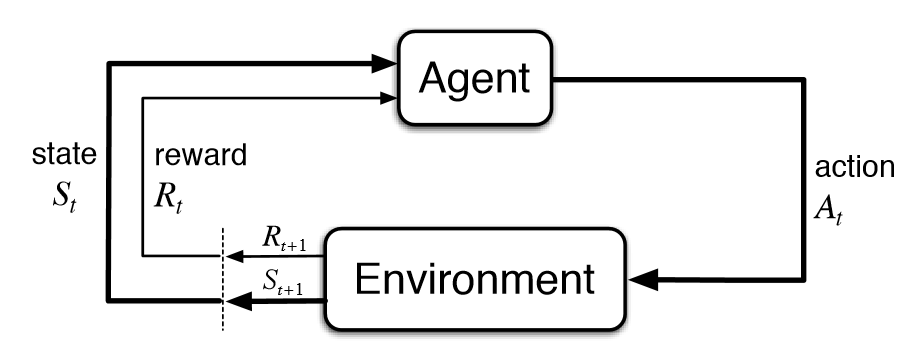
Now just how the agent actually learns in this setting is a consequence of several key components:
Component 1: An agent's policy defines the agent's behavior in any given state, and is typically represented by the Greek letter \(\pi\).
In general, the agent's policy is responsible for performing the mapping between state and action, though what constitutes a problem's state can differ from application to application.
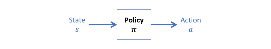
Designing this policy and how it changes in response to learning will be of intense focus in this course.
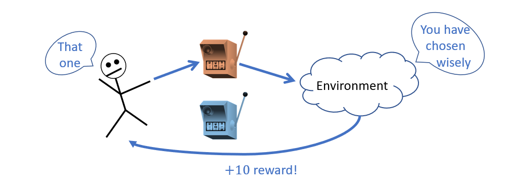
Component 2: the environment's reward signal defines the goals of the reinforcement learner providing feedback for actions chosen by the policy.
In almost all cases, the reward signal is a numeric value describing the utility of a particular choice, and has problem-specific value.
Some sub-properties of a reward signal:
It can be positive (encouraging that behavior) or negative (discouraging that behavior), mapping to biological analogs of pleasure and pain (respectively, except for any masochists in the audience).
It can have arbitrary magnitude such that larger rewards are preferable to smaller ones and larger punishments are to be avoided more than smaller ones.
Reward signals are sometimes within the control of the agent designer to set (to encourage / discourage specific behaviors) or may be outside of their control (the environment is not under the designer's influence).
These signals can also be stochastic functions of the environment's state and chosen action.
Note: the agent's sole objective in Reinforcement Learning problems is to maximize the cumulative reward it receives.
Everything the agent does and all designs of its policy are in pursuit of getting as much of that sweet sweet reward as possible.
Philosophy / Core Flag Scratching: are we as humans just chasing some arbitrarily complex rewards? O_O
Yet, the reward function provides the utility of an action in the short-term; what should an effective agent also learn to do?
Delay reward: if getting a *big* reward in the future means accepting lesser ones in the present, so be it, but an effective agent should be equipped to deal with this planning aspect.
This is also a big challenge: if you have a huge reward that is *distant* from an action that led to it, we have what's known as the attribution problem (a familiar one for anyone who has attempted to train a dog in complex tricks).
Or, you could ignore the above and simply end up with Hedonism Bot from Futurama, but for those who want a more rational agent, we need some measure of planning.
List some examples of reward signals.
Component 3: a value function maps a state to some future, cumulative reward an agent can expect to gain from that state into the future.
If the reward function provides the utility of immediate gratification, the value function considers the long term consequences of taking a particular action.
Note: rewards are primary in reinforcement learning tasks and values are secondary because the only purpose of the value function is in pursuit of achieving more reward!
Some notes on value functions:
Value functions are more difficult to reliably estimate than rewards because often an agent needs to explore actions and sample rewards before being able to accurately determine the value of a particular action and state.
Progress in this reliable estimation of value functions is what has driven the reinforcement learning field over the past 6 decades and led to some of the most impressive improvements in performance.
List some examples of hedonistic decisions vs. those that may be guided by a more pragmatic value function.
[Optional] Component 4: advanced RL agents may possess a model of the environment that can be used to mimic behavior of the environment and predict how actions will affect it.
Some bullets on the above:
Simple RL agents that do not have this component are known as model-free and are considered the "trial and error" opposite of model-based agents that can *plan* using these models.
Modern RL agents include both model-free and model-based agents, though (as that video from Pearl predicts) most practitioners agree that the field is headed toward the model-based approaches.
Indeed, integration of these models into RL algorithms is one of (in my opinion) the ripest opportunities for the incorporation of Causal Inference.
Whew! So, now that we've defined reinforcement learning within an inch of its life, let's look at its most fundamental application, some solution strategies, and where to go from there!
Multi-Armed Bandit (MAB) Problems
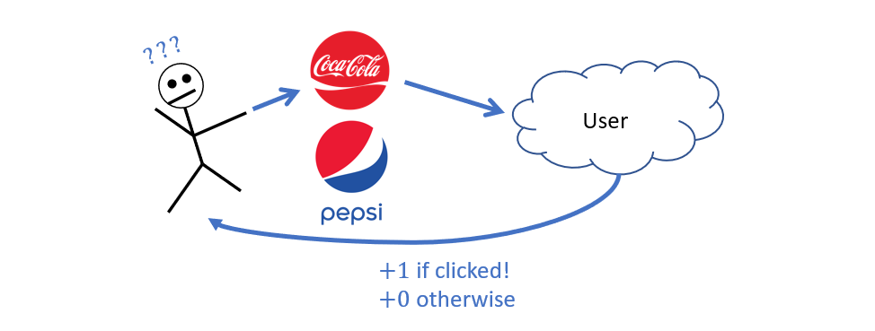
As our motivating example, consider an online advertising agent that must pick an ad to display to users visiting a page. When the ads are new, the agent must sample their efficacy before determining the best to show to different users.
For example, suppose Coca Cola decides to revive its old Coffee + Coke drink formerly known as Coke Black (RIP); some important questions for the ad agent:
Will an ad for Coke Black have a high chance of generating a clickthrough from teenagers? boomers? Southern Californians? etc.?
Will a *different* ad, e.g., for Pepsi (lol) have a higher clickthrough chance for those groups?
How should the agent figure out the answers to those questions?
It turns out that viewing this situation like a casino with different slot-machines, each of which may have different payout-rates is an apt analogy!
Problems of this type have been adorably named "Multi-Armed Bandit" problems and possess canonical set of properties.
Why the name "Multi-Armed Bandits?"
In the past, slot machines were known as one-armed bandits because they had an arm that you would pull to gamble, at which point they would steal your money (!)
In Multi-Armed Bandit (MAB) problems, an agent must maximize cumulative reward by sampling from some \(k \ge 2\) action choices (i.e., "arms") with initially unknown reward distributions in a sequential decision-making task. Specifically:
MAB agents make choices in a sequence of \(t \lt T\) trials for some (potentially infinite) Time Horizon \(T\).
In the simplest settings, at each trial \(t\), the agent makes some action choice \(A_t\) according to their policy, and receives a reward signal \(R_t\) from the environment, which then updates the agent's history for the next trial: \(H_{t+1}\).
Considering the simplest MAB problem in which decisions are independent of any environmental state or context, we can abstract the various trials into trial-subscripted components:
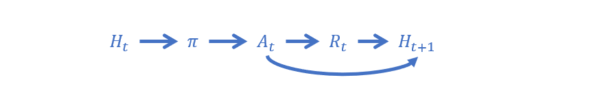
Things to note:
Above, the agent "learns" but updating its history with episodic memories from past decisions and rewards.
Future decisions are rendered independent from past ones by virtue of observing the current state of the history.
Looks pretty straightforward and simple... but why is this tricky?
Challenge: Sampling Bias
One of the biggest differences between vanilla causal inference and the problems we'll consider now are the issues brought about by having insufficient sample sizes.
Whenever we made CPTs in a Bayesian Network / HMM the general assumption is that (in the era of big-data) we have had near infinite data to confidently learn the network parameters to a good degree of accuracy.
However, in many RL domains, we may start from scratch and need to address innaccuracies that come from having finite samples of data, and how discovery must occur over the collection through time.
Consider the same example described above except made a bit more concrete: we have 2 slot machines / ads, \(X \in \{0,1\}\), that have different payout rates. Your task: find which one is the best! In class, we'll do this interactively.
Suppose in our first 3 samples of playing at each machine, we discover the following rewards:
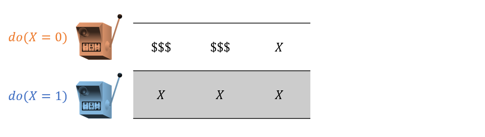
Which action would we want to exploit if we stopped exploring now?
\(X=0\) because it appears to have a higher win rate!
Suppose now, however, we sampled thrice more from each machine:
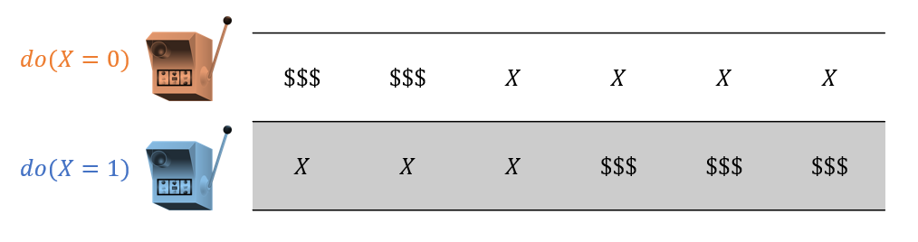
Now it looks like \(X=1\) is better!
This inadequate sampling can land us in trouble if we stopped trying \(X=1\) after getting 2 early wins with \(X=0\). This problem has a name:
Sampling Bias / Error can prevent accurate estimation of some query when noise and variance can contaminate small sample sizes.
Known as the Explore vs. Exploit dilemma, much of Reinforcement Learning centers around finding strategies that balance exploring the available choices with continuously exploiting the ones deemed best.
There are some risks here:
Explore choices too little and we may miss the optimal choice because we never saw that it was the best.
Explore choices too much and we may miss out on rewards that we would have gotten more of had we started exploiting sooner!
As such, solutions to the explore / exploit dilemma must take sampling bias into consideration.
So, let's consider the different ways we might implement this policy, and the different exploration-exploitation strategies that can be used in this simple MAB setting.
Action-Value Methods
Since, in MAB settings, our past actions neither change the state of the environments nor directly affect future actions, we are simply trying to find the best actions in the given context.
Action-Value methods thus assess the value associated with particular actions alone.
What would be the simplest means of computing the value associated with a particular action?
The average of rewards received in the past!
We can define this action-value as a sort of "query" on the agent's history such that for value of action \(a\) at trial \(t\) we have (from your text):
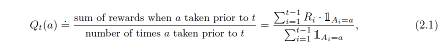
Some properties of our action-value \(Q_t(a)\) above:
The notation with the fancy looking \(1_{predicate}\) is called the indicator function which is 0 when the predicate is false, and 1 if true.
Its estimate of the action's rewards will be noisy and innaccurate until adequately sampled, lest it be infected by sampling bias.
Simple, though perhaps not the *best* way to assess the value of a particular action.
Action-Selection Rules
Although the action-value method gives us a target for assessing how good an action is in the past, we still need a policy that manages exploration and exploitation in the present.
An action selection rule (ASR) decides the policy's mapping from \(Q_t(a)\) to \(a_t\) in action-value methods.
Let's look at some of the most common action-selection rules and discuss their strengths / weaknesses.
I'll give you one to start:
ASR 1 - Greedy: The Greedy approach always selects the action with the highest current action-value: $$A_t = argmax_{a} Q_t(a)$$
Greedy indeed! This strategy attempts to maximize gains in the here-and-now, continuously exploiting what it presently believes is the best.
What is the major drawback of the Greedy ASR?
If the reward is stochastic, and the agent happens to get unlucky with what is (overall) the best action at the start, it may *never* select it again in the future!
That's a pretty big issue due to sampling bias!
Successful MAB agents should be able to guarantee that they will converge to the optimal policy if given enough trials.
So, with this new requirement in mind, can you consider a new ASR that would improve upon the Greedy?
Most people, when asked this question, will settle on one of the following techniques.
ASR 2 - \(\epsilon-\)Greedy is a simple amendment to the Greedy approach, which specifies that (at each trial) the agent will randomly choose an action with probability \(\epsilon\), and will exploit the current best via the Greedy approach with some probability \(1 - \epsilon\)
In plainer English, at each trial, we'll flip a biased coin: if it comes up heads (with probability \(\epsilon\)), we'll randomly choose an action to manage our exploration, and if it comes up tails, we'll choose the arm we currently believe to be the best.
To visualize this...
Draw the likelihood of an \(\epsilon-\)Greedy agent deducing the optimal action as a function of increasing trial, \(t\).
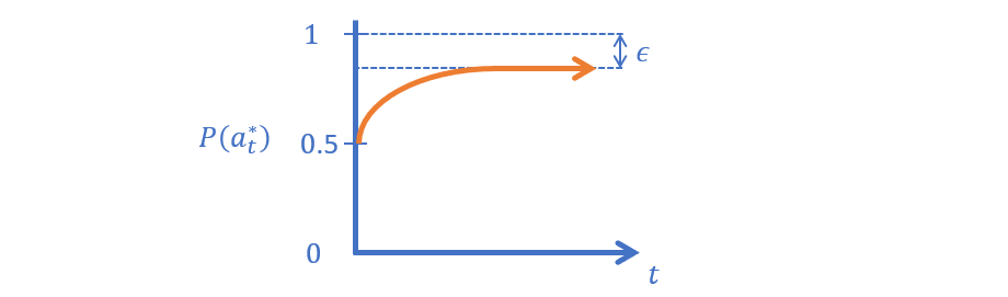
What's the problem with this method?
Even after the agent has discovered the optimal action, it will continue to perform costly exploration trials!
Can you suggest a remedy for this issue?
The next logical step may be to front-load the exploration!
ASR 3 - \(\epsilon-\)First randomly samples actions for the first \(n\) trials (for some choice of \(n\)), after which it exploits by the Greedy policy.
Draw the likelihood of an \(\epsilon-\)First agent deducing the optimal action as a function of increasing trial, \(t\).
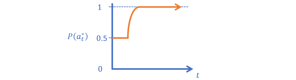
What's the problem with this method?
Three issues: (1) how to choose the threshold \(n\)? (2) how to guarantee that your sampling was sufficient to find the optimal arm if choosing randomly? (3) What if the optimal arm is obviously better than the others? Lots of wasted exploration that could have been spent exploiting.
To visualize this...
Is there a happy medium between these 2 ASRs?
ASR 4 - \(\epsilon-\)Decreasing is just like \(\epsilon-\)Greedy except that the value for \(\epsilon\) starts high and diminishes over time using some form of simulated annealing.
In other words, start off with a high chance of exploring, and then taper this propensity as trials go on.
While this seemingly offers a nice compromise between the previous ASRs, it still suffers from some of their theoretical constraints...
Draw the likelihood of an \(\epsilon-\)Decreasing agent deducing the optimal action as a function of increasing trial, \(t\).
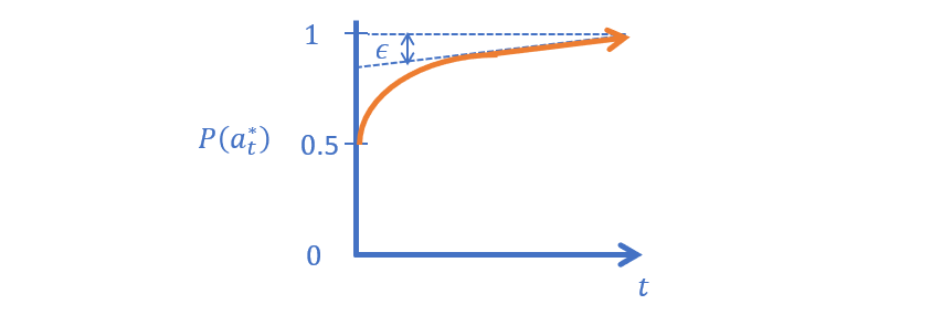
What's the problem with this method?
Two issues: (1) how to choose the decay rate? (2) how to guarantee that your sampling was sufficient to find the optimal arm during the time of decay?
More modern ASRs consider the agent's History from a Bayesian perspective, but use another tool we haven't yet talked about a lot.
A Probability Density Function (PDF) determines the probability... of a probability being the true chance of some event as concluded from a finite sample, with more variance associated with smaller samples!
Who better to tell us a little about PDFs than good old 1B3B? Watch up until the 6:00 mark:
How do PDFs help us think about crafting a MAB agent?
PDFs are functions used to represent the likelihood that a probability of some event is the true one. We can use a PDF to model the likelihood that the reward rate associated with each arm is the true one given finite-sample variance from our agent's history!
In brief:
This is useful for another reason from an old friend in 3300: sampling!
Sampling a value \(x\) from a distribution \(P(X)\) means to produce a simulated value \(x\) that is consistent with the underlying distribution and is written: $$x \sim P(X)$$
These more statistical techniques stem from several observations:
Observation 1: unless the reward distribution is non-stationary (i.e., changing over time), then there exists some "true" reward likelihood \(P^*(R|a)\) associated with each action \(a\).
Observation 2: initially, these true expected rewards are unknown, which we can encode as PDFs estimating \(\hat{P}(R|a)\) with high variance when they've been infrequently chosen, and then *sample* (i.e., get an estimated likelihood of reward probability) to get an approximation of their quality.
Observation 3: as arms are *chosen* more, the picture of their true expected reward gets more crisp, i.e., the PDF variance diminishes, and we can then reliably conclude which is best.
It turns out there's another statistical tool that can wrap up the above observations nicely!
ASR 5 - Bayesian Update Rule (AKA Thompson Sampling) is a "dynamic ASR" that maintains PDFs of each arm as models of their true success rates, with less frequently sampled arms having PDFs with higher variance. Its steps are generally as follows:
Once at the start: Initialize uniformly each PDF that estimates \(\hat{P}(R|a)~\forall~a\), the probability of reward \(R\) from chosing action \(a\).
-
For each sequential decision at trial \(t\) it makes:
Sample an estimated reward "quality", \(r_a\) from each arms' distributions: $$\hat{r_a} \sim \hat{P}(R|a)~\forall~a$$ Save all of those samples in a set / list called \(\hat{R_a}\) $$\hat{R_a} = [\hat{r_0}, \hat{r_1}, \hat{r_2}, ...]$$
Choose the highest of those samples as the next arm chosen, call that chosen action \(a_t\): $$a_t = argmax_{a} \hat{R_a}$$
Update \(\hat{P}(R|a_t)\) with the observed outcome, shrinking variance of expected reward around the chosen arm \(a_t\).
Suppose we have a 3-armed bandit problem between three arms, \(a, b, c\) (e.g., 3 ads) in which we have accrued some samples that provide the following distributions (known as Beta distributions for binary rewards) over expected reward (e.g., probability of clickthroughs).
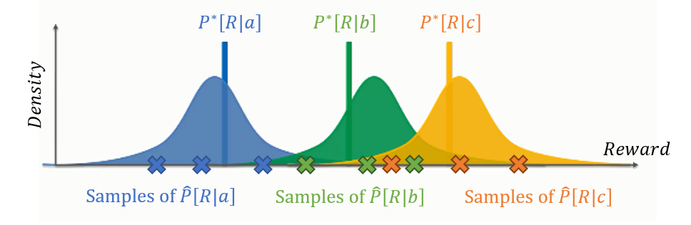
Image credit, my improvements.
Notes on the above:
The distributions as depicted have high variance, meaning this is likely the state of things early in the agent's lifespan.
Each X along the access is not an observed data point, but rather, a "sample" *from* the estimated reward distribution (the curves) to assess their quality while allowing inferior looking actions to still have a chance at being chosen in the early stages of exploration.
Samples are accomplished by "throwing a dart" in the area around the curve, which means that values closer to the average are more likely, but those in the tails are still possible.
As such, observe the interaction of 2 possible samples from the \(b, c\) actions in which one sample from \(b\) (the actually inferior arm) can be chosen over the superior arm \(c\) if we get unlucky with the sample from \(c\) but lucky with the sample from \(b\).
Plainly, then, we would like these distributions to change as the agent gets experience. Consider now that some time has passed, and the variance on more-likely sampled distributions diminishes:
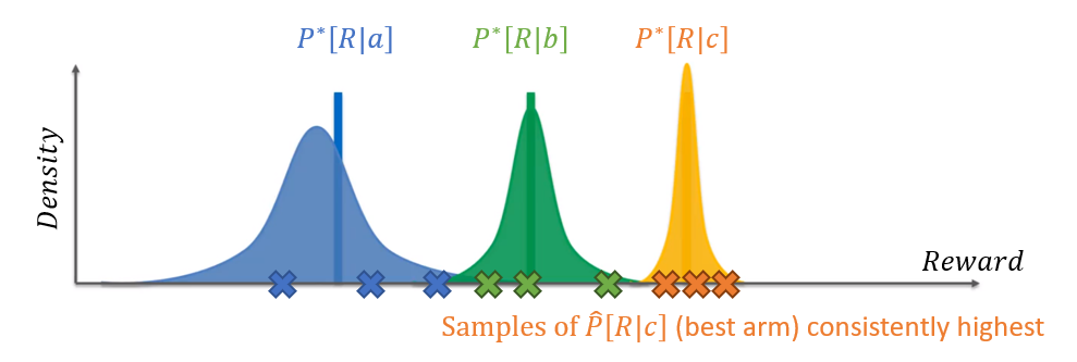
Notes on the above:
As more and more samples are collected from the top arms, their variance diminishes, and the cases like getting "unlucky / lucky" with certain samples as described above become nonexistent.
From this point on, the best arm is chosen, confident that others have been sufficiently explored.
Why, then, did the blue distribution above (action \(a\)) not have its variance decreased as much as the other two?
Because its samples were likely much lesser quality than the other two, and so it remained relatively unexplored. Still, we didn't need to explore it more, because its quality was so much lower.
Note: this means that the only arms whose true reward rates are ever discovered are typically the optimal -- others are left insufficiently sampled, which is actually a good thing.
Take a look at some MAB animations, including how the distributions with Thompson Sampling change with samples!
And there you have it! A first look at Reinforcement Learning with some great theoretical foundations, and example implementations.
Next time, we make things a bit trickier...