Last week we saw our Infamous Firing Squad example to illustrate the use of counterfactuals, but far be it from me to let such a gratuitously violent motivating example die out in a single lecture.

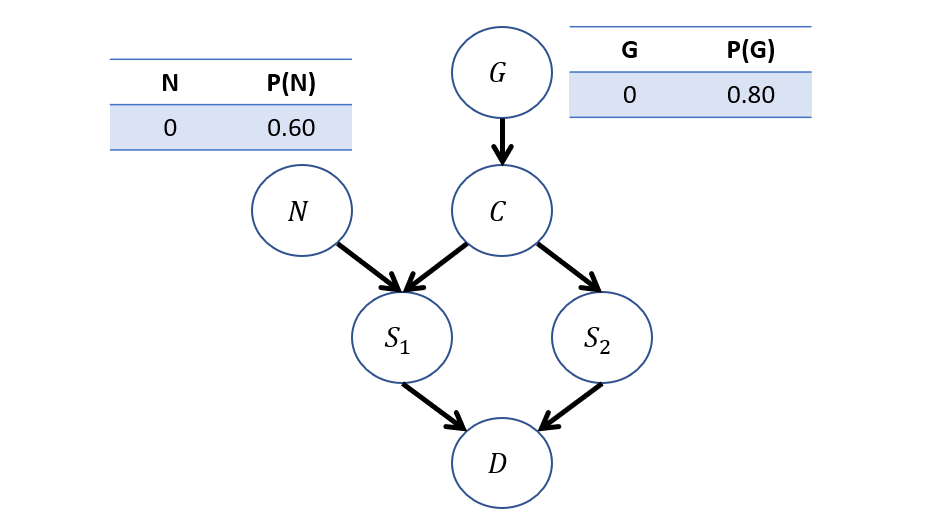
Suppose now, we modify our Firing Squad example to model the Nerves (N) of the flunky Soldier 1, which may cause him to fire on accident despite the captain's orders:

\begin{eqnarray} M:\\ U &=& \{G, N\} \\ V &=& \{C, S_1, S_2, D\} \\ P(u) &=& \{P(G=0) = 0.8, P(N=0) = 0.6\} \\ F &=& \{ \\ &\quad& C \leftarrow f_c(G) = G \\ &\quad& S_1 \leftarrow f_{s_1}(C, N) = C \lor N \\ &\quad& S_2 \leftarrow f_{s_2}(C) = C \\ &\quad& D \leftarrow f_{d}(S_1, S_2) = S_1 \lor S_2 \\ \} \end{eqnarray}

The now updated graphical model, with CPTs:

Let's revisit our counterfactual query from last time: "What's the likelihood that the prisoner dies if \(S_1\) doesn't shoot, given that he did?" $$P(D_{S_1 = 0} = 1 | S_1 = 1)$$

Crucially, what changed in this problem from how we answered this query last time?

Our update to the exogenous variables now has to take into consideration that, observationally, \(S_1\) may have shot because he got the order OR because of nerves.

Drawing the twin network model for this query gives us:

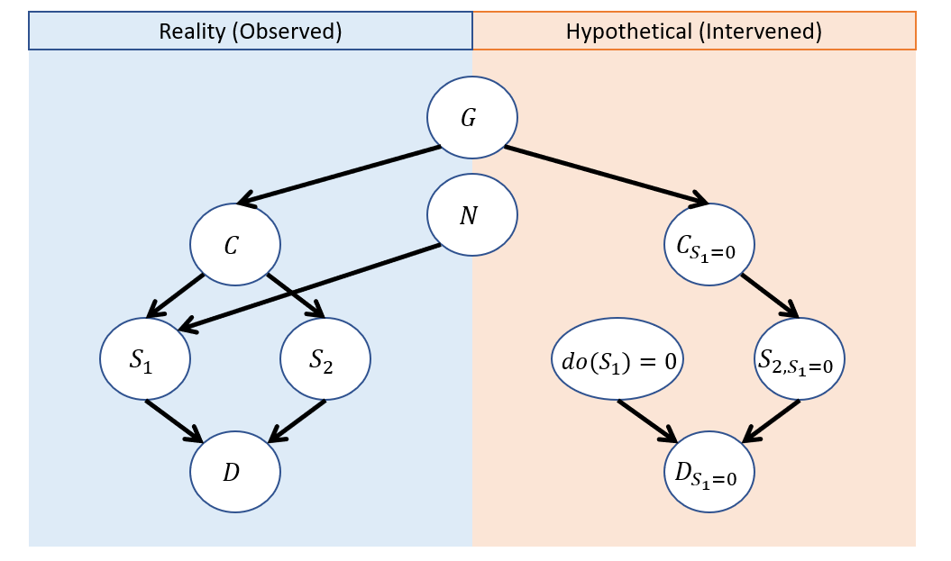
Why don't we draw an edge between \(N\) and \(do(S_1)\) in the hypothetical model?

Because we are performing the do operation on \(S_1\) to compute our hypothetical -- \(N\) has no power here!

So, let's see how we go about performing our 3-step counterfactual computation:

Abduction: Update \(P(U) \rightarrow P(U|e)\).

In general, we would have to update the distribution of all \(U\), but in this particular instance, which is the only we must update and how?

Just \(P(G) \rightarrow P(G|S_1 = 1)\) because \(G\) is the only \(U\) shared between the observed and hypothetical worlds!

We can, in just the observed model, perform this by deriving the CPTs on each \(V\) as they'd be uniquely decided by \(\langle P(u), F \rangle\)!

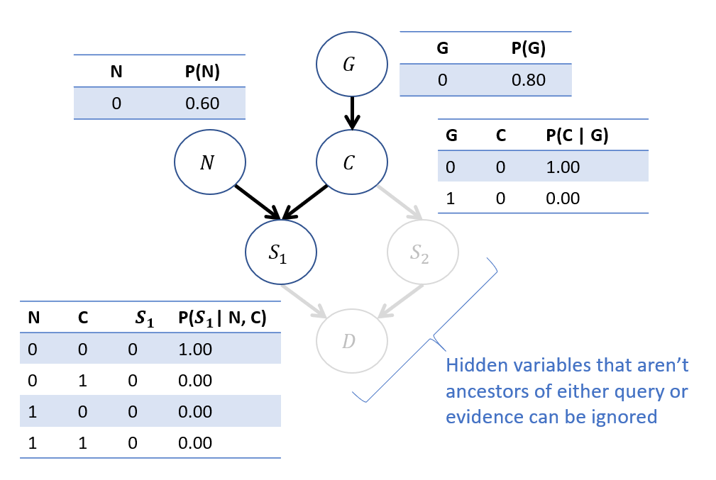
Performing this update using our typical tricks:

Step 2 - Action: Switch to interventional model \(M_{S_1 = 1}\) with updated \(P(U)\).

Note below our new CPT on G in the interventional model! This was the result of abduction.

Step 3 - Prediction Solve for \(P(D_{S_1 = 0} = 1)\) in interventional submodel.

This is left as an exercise, but intuitively we can work out:

• The only way the prisoner dies in this world is if \(S_2\) shoots.

• \(S_2\) will only shoot if the Captain gave the order.

• \(C\) only gives order if prisoner is guilty.

• In this world, the prisoner is guilty \(P(G=1) = 0.38\) of the time.

Therefore, we achieve the answer to our original query:

$$P(D_{S_1 = 0} = 1 | S_1 = 1) = 0.38$$

Jesus... what a ride.

As we've seen, counterfactuals are nifty and answer some interesting query questions...

However, sometimes we may have counterfactuals of interest but cannot compute them for a variety of reasons.

Consider some reasons why we might not be able to compute a counterfactual of interest.

• For counterfactual \(Y_x\) The causal effect of the antecedent \(x\) on the query \(Y\) may not be identifiable given our data (maybe we have only obs. data).

• Perhaps we lack, or are unwilling to honestly assume, any type of SCM (fully- or partially-specified) to explain the system.

In cases like these, we cannot lean on some of our algorithmic approaches to counterfactual computation, but might be able to salvage some anyways.

Let's consider a motivating example:

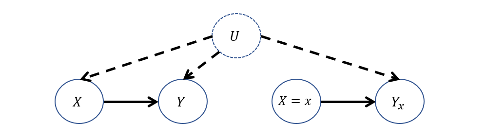
Let's revisit our drug trial example wherein one of two treatments \(X \in \{0,1\}\) are typically used to treat some condition, after which patient recovery \(Y \in \{0,1\}\) is observed. Moreover, doctors tend to prescribe each of these different treatments as a consequence of some unobserved factors that may reflect personal preference or other features that also happen to related to recovery, giving us the model:

Suppose we wish to compute the likelihood of recovery for prescribing an alternative treatment (WLOG, \(X = 1\)) to what was given in reality (WLOG, \(X = 0\)), a counterfactual of the format: $$P(Y_{X=1} = 1 | X=0)$$

Consider the Twin Network Model associated with this query: why would computing \(P(Y_{X=1} = 1 | X=0)\) be difficult here?

Since all nodes in the interventional side are dependent on the counterfactual antecedent, we don't have a clear way to perform abduction! Moreover, if we only had observational data, the interventional effect is not identifiable.

To visualize, that network would look like:

Still, all hope is not lost; suppose we have in our possession both observational data \(P(Y|X)\) from examining these treatment outcomes in physicians' practices, and experimental data \(P(Y|do(X))\) from some FDA study.

It turns out that having this data in this setting is alone enough to answer our counterfactual query -- all through the power of simple probability calculus!

Let's see how that works:

In settings with binary treatment \(X\) and in possession of both observational and experimental data, the counterfactual \(P(Y_{X=1} | X = 0)\) is estimable via the equation: $$P(Y_{X=1} | X = 0) = \frac{P(Y_{X=1}) - P(Y | X = 1)P(X = 1)}{P(X = 0)}$$

Neat trick! A bit limiting since we are bound to only binary treatment; a constraint we will see can be loosened with other methods in a future section.

This data-driven approach to counterfactuals has led to some other important queries that are often termed "practical" counterfactuals, since they have certain common interpretations across disciplines, like in medicine, philosophy, and others.

We'll look at a select few of these now.

Probability of Necessity / Sufficiency

---

Causality discusses the notion of "blame" or "attribution" in counterfactual terms!

• Was a cause necessary to elicit some effect (i.e., an effect *can only* happen in the presence of the cause)?

• Was a cause sufficient to elicit some effect (i.e., an effect happens *whenever* the cause is present)?

The notion of "present" or "absent" generally casts these questions of blame / attribution as binary variables: 0 = absent, 1 = present.

These two questions have counterfactual formalizations:

The Probability of Necessity (PN) is computable for outcome \(Y\) and treatment \(X\) by: $$PN(X \rightarrow Y) = P(Y_{X = 0} = 0 | X = 1, Y = 1)$$

Consider if \(Y=1\) headache cured and \(X=1\) took aspirin. If you took aspirin \(X=1\) in reality and your headache went away \(Y=1\), then we could ask what the probability would be of still having the headache \(Y=0\) in the world where we DIDN'T take aspirin \(X=0\).

If \(P(Y_{X = 0} = 0 | X = 1, Y = 1) > 0.5\), it's more probable than not that the aspirin was necessary for the headache to go away, otherwise, in its absence, it might've gone away anyways!

In words, "What is the likelihood that the effect \(Y\) would not have happened in the absence of \(X\), given that it did when \(X\) was present?"

Necessity is just one part of "blame" or "attribution," the other being:

The Probability of Sufficiency (PS) is computable for outcome \(Y\) and treatment \(X\) by: $$PS(X \rightarrow Y) = P(Y_{X = 1} = 1 | X = 0, Y = 0)$$

In words, "What is the likelihood that the effect \(Y\) would have happened in the presence of \(X\), given that it did not when \(X\) was absent?"

Consider a social justice application in terms of hiring practices: if a company is facing scrutiny in age-ist hiring practices (e.g., only hires young applicants), consider how one of the tools above could be used to ensure the company is held accountable for bias.

We could examine hiring records to estimate the probability of sufficiency where: $$PS(X \rightarrow Y) = P(Y_{\text{young}}=\text{hired}~|~\text{old}, \text{not hired})$$

Blame and attribution take on a compellingly intuitive definition in this format: "Would the candidate have gotten the job *had they been* young?"

A "more probable than not" (i.e., over 0.5) result may yield a basis for legal action!

Lastly, one quantity that is sometimes referred to as a "true cause" combines the above:

The Probability of Necessity and Sufficiency (PNS) is the likelihood that some treatment \(X\) is both necessary and sufficient to elicit some outcome \(Y\). $$PNS(X \rightarrow Y) = P(Y_{X=1}=1, Y_{X=0}=0)$$

Imagine the twin network(s) for the above! Kinda crazy!

Note: PN, PS, and PNS all have meaningful bounds for estimation in lieu of a fully-specified model and can be estimated from data alone -- we won't explore those here, but you can find more info in your textbook's final chapter!

Where have we seen the notion of "attribution" before, and why might the above be useful?

In reinforcement learning, the "attribution problem" was one in which it was difficult to determine the "reason" for a received reward, and so certain features may be *misattributed* to it, causing problems.

Effect of Treatment on the Treated (ETT)

Consider our past examinations in differences between certain queries in each layer of the causal hierarchy.

At the observational layer, we could ask for the risk difference (RD) in some patient's recovery rates across different treatment options, as governed by the equation:

$$RD(X \rightarrow Y) = P(Y = 1 | X = 1) - P(Y = 1 | X = 0)$$

Risk difference assessed the associated, though not necessarily causal, difference in some outcome metric from different observed treatments.

At the interventional layer, we could ask for the average causal effect (ACE) of one treatment on recovery over another:

$$ACE(X \rightarrow Y) = P(Y = 1 | do(X = 1)) - P(Y = 1 | do(X = 0))$$

The ACE assessed the causal difference in the average population of one treatment over the other.

Following this trend, what practical quantity logically follows for the counterfactual layer, given that its motivation was to find more individualized treatment effects?

The difference in recovery rates of what treatment *was given* vs. what treatment *could have been* given.

This quantity is well known in many disciplines as the Effect of Treatment on the Treated and is specified as follows.

The Effect of Treatment on the Treated (ETT) provides the difference in some outcome of interest \(Y\) between a treatment hypothesized \(X = x\) that is different than one that was assigned in reality \(X = x'\), and is computed by: $$ETT = P(Y_{X = x} | x') - P(Y_{X=x'} | x') = P(Y_{X = x} | x') - P(Y | x')$$

The ETT can inform us of cases wherein we need to assess whether a treatment policy that is enacted in reality is optimal compared to potential alternatives.

Let's see an illustrative example from the book (and finally something that doesn't involve firing squads, cancer, or worse, exercise).

In order to assess the efficacy of the program *post-launch,* why might the ACE not be the right tool given that participants self-enroll?

Because those who self-enroll into the program may be more resourceful, socially connected, and/or intelligent than those who do not, and so these individuals may have gotten jobs *with or without* the help of the program!

Note that potential confounds like resourcefulness or intelligence get washed out between experimental conditions in the randomized trial, so we would not necessarily know about differences introduced by these traits from the interventional data / tier.

As such, in order to assess the efficacy of the program in practice, we would need to find a means of computing the ETT using a combination of observational and experimental data like through the technique that we outlined above.

In words, what would the ETT computation tell us for the unemployment training program above? $$ETT = P(Y_{X=0}=1 | X=1) - P(Y=1 | X=1)$$

This provides the *differential* benefit of the program to those enrolled: the extent to which hiring rate has increased among the enrolled compared to what it would have been had they not trained.

Some possible outcomes of the ETT:

• [Helpful] If negative, then participants would have faired worse had they not participated.

• [Ineffective] If zero, then those who participated in the training were no better served than had they not.

• [Harmful] If positive, then participants would have faired better had they not participated.

We'll see the ETT help us in another practical setting shortly!

In the previous tiers of the causal hierarchy, we saw empirical means of sampling / collecting data that provided qualitatively different implications with the questions that each type of data could answer.

The empirical sampling strategies of the first tiers of the causal hierarchy are well practiced, including random sampling for observational data, and random assignment / experimentation for interventional data.

Reasonably, we might wonder: is there an analog for *empirically* collecting counterfactual data?

This very question sounds laughable -- why?

Because "empirical" means "factual / witnessable" and we're asking for a witnessable way to measure something that runs contrary to reality!

Surprisingly, we actually *can* measure some counterfactuals empirically, even when we don't possess a fully-specified model, even when there is unobserved confounding present, and even when we have more than 2 treatments / actions to consider!

Here's how...

The Utility of Intent

---

Consider again our confounded decision-making scenario with physicians prescribing a wider variety of treatments \(X \in \{0, 1, 2\}\) with the objective of maximizing recovery rates \(Y = 1\), but in the presence of confounding factors.

Objective: determine, for each alternative treatment, the likelihood of recovery compared to the one given, i.e., compute: $$P(Y_{X = x} = 1 | X = x')~ \forall~ x, x' \in X$$

This is a particularly difficult challenge because:

• We do not possess the fully-specified SCM to answer this counterfactual.

• There are confounding factors present between \(X, Y\) for which we cannot outrightly control.

• Even if we had both observational and experimental data, we can't use our trick from the first part of this lecture because \(X\) is not binary!

However, we can exploit the following insight:

Decision-making is a two-step process: (1) Developing an intended action as a response to environmental factors (observed or unobserved), and (2) enacting that decision.

Separating any decision into these two steps (intent and enaction) allows for the observed, intended action to serve as a proxy for the state of any confounding factors, in which the effect of some intervention can be predicted.

Modeling this 2-step decision process explicitly, our model becomes:

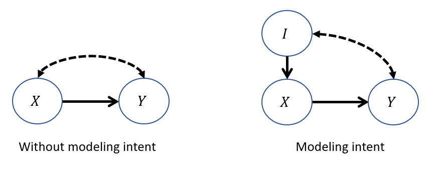
Above, we have a physician's intended treatment \(I\) modeled as an observed parent of their finally enacted treatment \(X\).

• Observationally: The intended treatment will always be the same as the enacted.

• Interventionally: The enacted treatment will be independent from the intended.

• Counterfactually: We can examine the treatment's interventional effect when it *disagrees* with the intended.

Why is explicitly modeling the intent useful for this third, counterfactual query?

Because an actor's (physician's) intended treatment provides information about the state of the unobserved confounders, which in turn provides more information about the efficacy of treatments under that context. Intent is back-door admissible for the effect of \(X\) on \(Y\)!

Intuition: Have you ever tried to break a bad habit? Your *intent* desires a particular action (the habitual) that you then *override* to choose differently!

What topic from reinforcement learning is this a lot like?

Policy Iteration! If your current policy \(\pi\) selects an action that is worse than another hypothesized, update that policy!

So, how do we now translate this insight to measure these counterfactuals at scale?

Counterfactual Randomization

---

Counterfactual Randomization describes any procedure in AI / the empirical sciences by which the outcome of a randomly chosen decision is compared to a decision that would have happened without that randomization on a single unit / patient / moment in time.

The Confounded Physicians: consider a scenario in which two or more Physicians (or generally, actors [not like, Doogie Howser, but some agent making an action]) are treating patients but are subject to unobserved confounders between treatment selection and outcome (e.g., direct-to-consumer drug advertising or perceptions of patient SES). Each has different policies \(f^{A_1}, f^{A_2}\) which may cause them to respond differently, and we need to scrutinize these policies for how they perform in practice.

• Shockingly, given the same patient, there is ample evidence of marked variance in how those two physicians would choose to treat!

• Any drug will still have to be vetted through a traditional FDA Randomized Clinical Trial (RCT), so we need not tinker with that methodology.

• However, on top of randomly assigning each participant to an experimental condition, we can also collect a panel of actors' (i.e., physicians') intended treatments for each patient, which (importantly) may disagree with the one randomly assigned.

Consider now a new Counterfactually Randomized procedure that combines random sampling with random assignment. In particular:

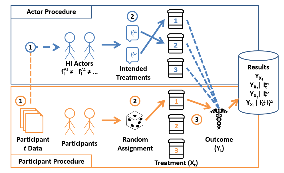
Interpreting the results of an HI-RCT yield some really rich findings that other empirical methods may miss:

• Experimental data [\(P(Y_x)\)]: since the RCT component (bottom panel) of an HI-RCT is untouched, we can simply ignore any actors' intents and still have interventional data from the random assignment.

• Observational data [\(P(Y | X)\)] whenever the randomly assigned \(X\) and an actor's intended treatments *agree*, we've generated (by the consistency axiom) an observational data point.

• Counterfactual data [\(P(Y_{X = x} | X = x')\)] whenever the randomly assigned \(X = x\) *disagrees* with an actor's intended treatment \(I = X = x'\), we've generated a counterfactual data point!

Neat!

It turns out this procedure, and the accompanying analytics, are hot off the presses (Forney & Bareinboim, 2019). Yeah that's right, I made this.

The implications and applications are yet to be tested except in theory, and leave a ripe opportunity for future research into how we can evaluate actors' policies, either human or artificial, in pursuit of finding those for which no alternative action than the one given is regretted.

Reflect: how else might this technique map to some human cognitive process and its automation for artificial agents? What utility might this serve for an AI?

Whew! Another action-packed day in causality! Next time: a final class of SCMs that have some interesting properties.