By this point, we've seen some really important causal models and the cool tricks we can do with them, including:

• Causal Bayesian Networks (Unlocked Tier 2 of Causal Hierarchy)

• Partially- and Fully-Specified Structural Causal Models (Unlocked Tier 3 of Causal Hierarchy)

Although at the top of the food chain, there're probably a couple of burning questions you might have about SCMs, and in particular, how we can deploy these in practice on real data...

What are some of the less practical aspects of the SCMs we've been using up until now?

Several primary issues: (1) where do the functions come from when we don't know them, and (2) how do we know when to model exogenous variables as independent or not from one another, and (3) what if we have causal effects that aren't discrete?

To at least try and solve them, we'll lean on a few traditional tools from those same sciences, and see how we can adapt them to our goals of forming SCMs that can still answer queries at all tiers of the causal hierarchy.

Let's start with a motivating example.

Consider that we wish to study the causal relationship between \(X\) = weekly hours in an afterschool program, \(Z\) = weekly hours doing homework, \(Y\) = difference in quality points (i.e., GPA * Units) from before afterschool program.

Handwaving some causal discovery questions for now, there's reasonable precedent to suppose that the causal structure between these variables is as follows:

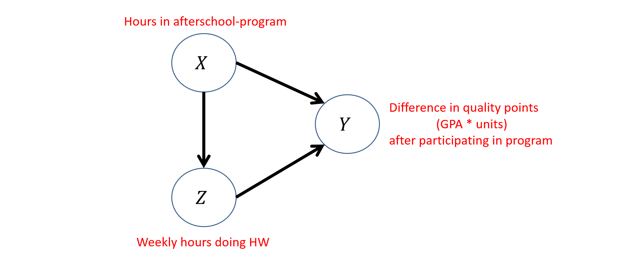
Yet, there are some interesting questions that we must answer to be able to use such a model for this problem:

1. How to represent and / or learn structural equations? Since we don't have these to start, perhaps they can be estimated...

2. How to translate our past tools to continuous variables? E.g., we might be interested in how effective an additional 1.25 hours of study is vs. 1.5 -- we can't really use discrete CPTs any longer to perform inference!

3. How to test for dependence / independence with continuous vars? Before, our definitions were in terms of probabilities, but how does that scale now?

4. How do we perform inference with all of the above?!

Borrowing from Regression

---

Recall one of our early examples from the first lectures in which we examined an association between housing prices and square footage:

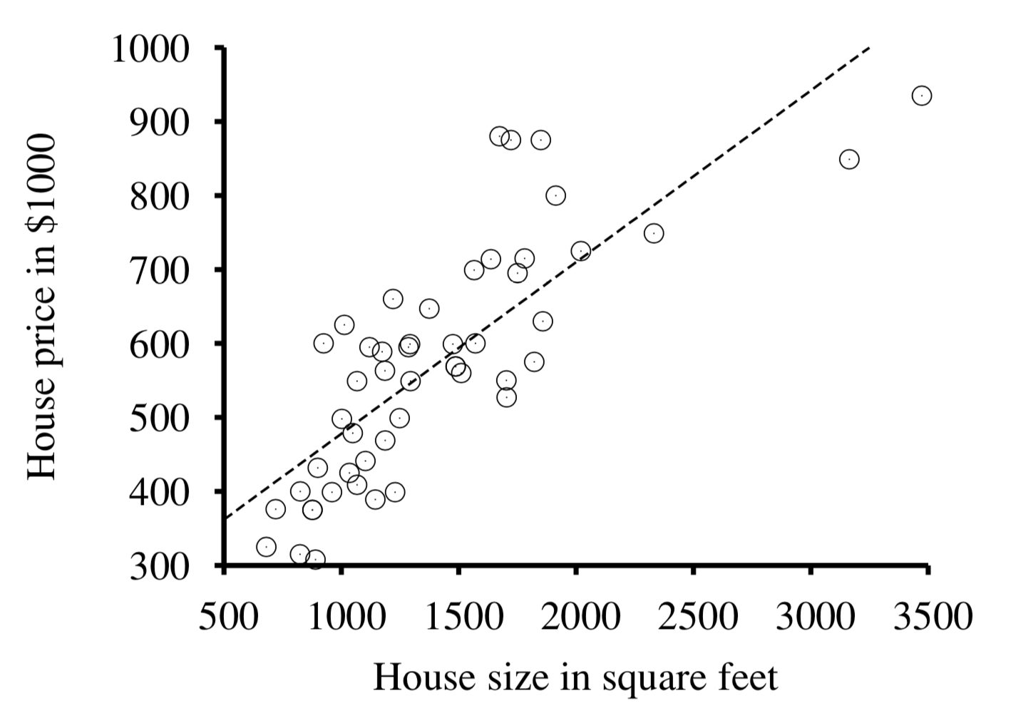
Noticing the dashed regression line (i.e., the line of best fit for the trend), how might we be inspired to use a similar tool in pursuit of addressing our primary issues above?

Use the regression equation as an empirically estimable structural equation!

In other words, if we are to defend that the relationship between some \(X, Y\) is causal such that \(X \rightarrow Y\), we can envision: $$Y = m*x + b = \{\text{strength of X's effect on Y}\} * \{\text{value of X = x}\} + \text{disturbance}$$

Warning: regression is still an associative tool, but much like CBNs, when the causal structure is asserted, it can be used to estimate the relationships between causes and effects!

That said, there are some key differences with just regression coefficients (the slope) and how we use them in pursuit of causal inference, and that discussion starts with a little lesson in stats...

So quick, I didn't even have time to write out "statistics!"

Given the above reliance on some more traditional statistical ideas, we'll need a quick review of the tools we'll use in this final type of SCM.

Expectation

---

Hopefully yours are great!

This is one of the most basic ideas in stats with continuous variables: the average, or expected value.

When you think about it, the way we typically compute averages is just a special case of this idea, e.g., the average of some list of values \(X = [1, 5, 3, ...]\):

$$\mu_X = \frac{\text{sum of vals}}{\text{num vals}} = \frac{\sum_x x}{n} = \sum_x x * 1/n$$

We can rephase this slightly to get things into terms with which we're more familiar:

The expected value of some random variable \(X\) is its likelihood-weighted sum of values, defined as: $$E[X] = \sum_{x \in X} x * P(x) = \mu_X$$ ...where \(\mu_X\) is shorthand for the Expected Value of X.

The most basic example: let \(X\) be the result of rolling a six-sided dice with each side being its value and equal likelihood.

$$E[X] = 1 * \frac{1}{6} + 2 * \frac{1}{6} + 3 * \frac{1}{6} + 4 * \frac{1}{6} + 5 * \frac{1}{6} + 6 * \frac{1}{6} = 3.5$$

Expectation Property 1: This definition can be extended to conditionals as well, such that: \(E[Y | X=x] = \sum_y y * P(Y=y|X=x)\)

In fact, you can put whatever function of some \(X\) in the expectation and get the expected value, e.g., \(E[g(X)] = \sum_{x \in X} g(x) * P(x)\)

We'll use the expectation \(E[...]\) notation quite a bit in the lectures that come, and you'll see it crop up a lot outside of this class too.

Expectation Property 2: The \(E[c] = c\) for some constant \(c\) is just that constant!

Expectation Property 3: The linearity of expectation is the property that the expected value of sums of variables is the same as the sum of their individual expectations: $$E[Y + X] = E[Y] + E[X]$$

We'll make use of this later!

Variance

---

Close on the definition of expectation is that of variance: if expectation tells us the average, then variance tells us the "spread" of the data, i.e., how close some sample or population is to the average.

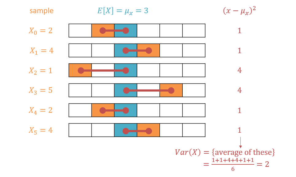
Variance of some variable \(X\) is the expected squared distance of its values from its average, \(\mu_X\), viz. $$Var(X) = \sigma_X^2 = E[(X - \mu_X)^2] = \sum_x (x - \mu_X)^2 * P(x)$$

Some notes on the above:

• Note that we square the error for a couple of reasons: (1) without it (since we're summing over the difference of all values and the average), we would just get a sum to 0, and (2) higher deviances are penalized more (plus, it's just mathematically convenient to deal with squares than absolute values).

• Much like expectation, the above can be performed for either an analytic event (whose states and likelihoods are known, like a dice role) or dataset (i.e., a sample) over \(X\)

By squaring the differences between each \(X=x\) and \(\mu_X\), we are no longer in the same units as the original \(X\), so often, we want to instead examine the standard deviation, the square-root of the variance: $$SD(X) = \sigma_X = \sqrt{\sigma_X^2}$$

Most variables / data exhibit a normal distribution ("the bell curve") with sample mean centered around the population average and roughly equivalent standard deviations, which has nice properties:

Blurry image credit to Wikipedia.

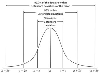
Since, in causal inference, we usually are operating under assumptions of large sample sizes (to avoid the pitfalls of sampling bias that we've seen earlier in the semester), and that we endeavor to account for as many causes of an endogenous variable as possible, normality of our variables / distributions is generally assumed.

Note that some corrections usually need to be taken if our data isn't normally distributed (a typical way to deal with skewed data is to take its log, which then becomes normally distributed with some careful correction), but for this introduction, we'll assume that ours is.

One of the (many) niceties from assuming normally distributed data is the ability to express variables in standardized values:

Standardized- / Z-Scores are ways of expressing some variable's value as the "number of standard deviations above (positive Z-score) or below (negative Z-score) the mean." $$Z = \frac{x - \mu_X}{\sigma_X}$$

We'll make use of these later as a convenient way to express certain causal relationships.

Covariance

---

Of course, in any causal endeavor, we don't just care about the descriptive statistics surrounding one variable, but moreso what variables tell us about others!

As such, we will primarily care about the way that two or more variables... well... vary *together*:

The covariance of two variables \(X, Y\) is the degree to which they vary together: $$Cov(X, Y) = \sigma_{XY} = E[(X - E[X])(Y - E[Y])]$$

Intuitively, looking at the formula above, if X and Y have large deviations from their average *at the same time* (i.e., for the same data point), then their covariance should have higher magnitude as well.

What are the possible signs / values of the covariance between two variables and what do those possibilities mean?

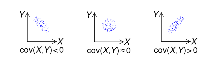
Note that IF two variable are independent, THEN their covariance will be near 0... but if covariance is near 0, they are only LIKELY to be independent, but certain non-linear relationships between variables can make for exceptions.

So how do the above ideas help us in causal inference? How the hell did we get here?

Just a little more, almost there!

Linear Regression

---

Linear Regression is a tool to determine what degree one variable's value predicts another, which is typically done (in empirical sciences) as a linear function for simplicity and to avoid overfitting.

Consider two dice rolls, \(X, Y\), the sum of those \(S = X + Y\), we wish to determine the best way to estimate \(E[S|X]\), and that we have a sample of \(N = 10\) rolls distributed as follows:

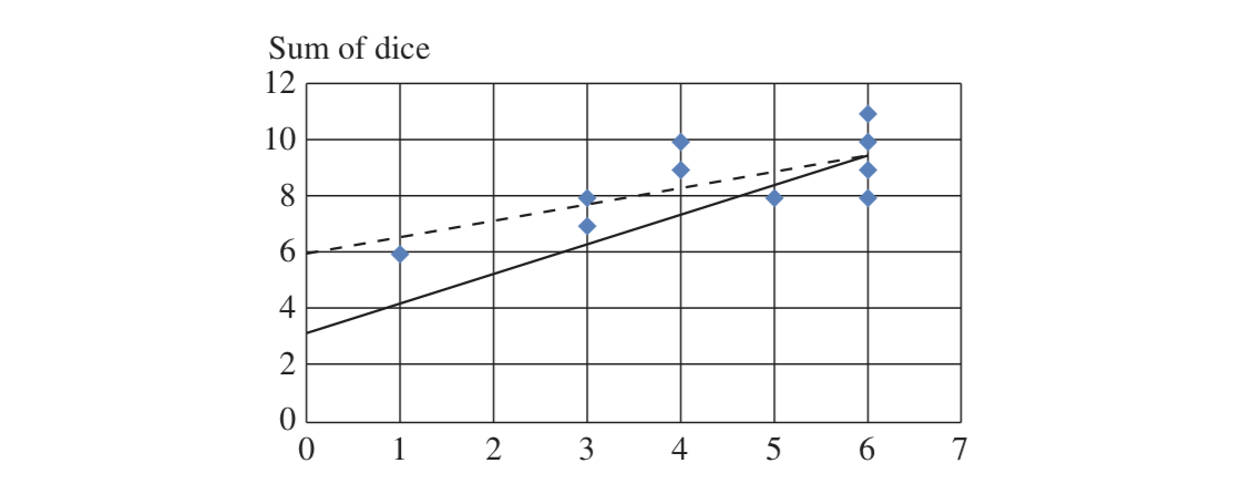
The above represents a scatterplot in which the blue dots represent dice rolls, and two regression lines pertaining to the population and sample.

In statistics, a population is the theoretical full / infinite dataset under study, and a sample is some subset of data points from the population. As the size of the sample \(N \rightarrow \infty\), the sample stats trend to the population ones.

So, in our dice example above, we could analytically derive the population regression line such that:

$$E[S|X=x] = E[Y + X | X=x] = E[Y | X=x] + E[X | X=x] = E[Y] + x = 3.5 + 1.0x$$

Note that the equation \(3.5 + 1.0x\) fits the equation of a line, and is indeed the best prediction line (shown in solid black in the figure above).

So, how do we estimate our sample regression line when we don't have an analytic / algebraic way of deriving it?

Least-Squares Regression is an optimization technique wherein for \(n\) data points (x, y) on our scatter plot, and for any data point \((x_i, y_i)\), the value \(y_i'\) represents the value of the line \(y = \alpha + \beta x\) at \(x_i\), then the least squares regression line is the one that minimizes the value: $$\sum_i (y_i - y_i')^2 = \sum_i (y_i - \alpha - \beta x_i)^2$$

Warning: serious handwaving here, there's a big discussion we don't have time for with regards to how regression coefficients are found and under what conditions.

Here's one fun tidbit: the proof that the Least-Squares Regression definition is the best linear fit for some data as long as there are no UCs in the system is known as the Gauss-(wait for it)-Markov Theorem. He's back, baby!

For the univariate regression case above (and left as an exercise / reading your textbook to rationalize):

In Multiple Regression, the goal is to find the best estimate for the partial regression coefficients \(r_i\) of multiple predictors \(X_i\) on a single variable of interest \(Y\): $$Y = r_0 + r_1 X_1 + r_2 X_2 + ... + r_k X_k + \epsilon$$

The ways of finding each of the \(r_i\) above aren't trivially derived analytically, but all you need to know is that there are efficient Least Squares solvers to determine the best values for them that maximally predict the value of \(Y\).

Important to us in causal inference: how do we harness regression in pursuit of enriching or enabling our SCMs?

To recap:

• Knowing the exact structural equations that decide our endogenous variables is often very difficult, but we'd instead like some estimate for them to use the cool tools we've been talking about.

• Linear Regression lets us estimate how well one or more variables predict another, and provide linear equations that can be fit from data.

• These might not be as good as the actual structural equations, but are good estimates!

So, let's look at how to formalize our new type of SCM and then how to use them in a funky fresh kind of inference.

Pretty much everything else is the same!

Here are the key differences:

• Instead of inferences over probability values \(P(...)\), we're instead examining expectations \(E[...]\)

• The rules of d-separation still apply, so for example, if our structure is \(X \rightarrow Z \rightarrow Y\), then \(E[Y|Z,X] = E[Y|Z]\) because \(Y \indep X | Z\).

• Along each edge in the graphical structure, we represent a path / causal coefficient depicting the amount by which the child's value increases with each unit-increase (i.e., increase by 1) of the parent.

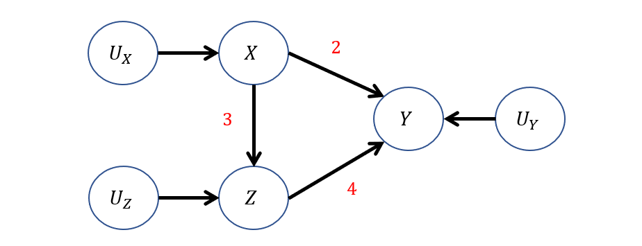
Back to our GPA intervention modeling goal from before, let's now complete its representation as a LSCM supposing we used regression to derive the following LSCM structural equations (the precise details of finding each I'll handwave for now):

\begin{eqnarray} M:\\ V &=& \{X, Z, Y\} \\ U &=& \{U_X, U_Z, U_Y\} \\ E(U_i) &=& 0~ \text{AND}~U_i \indep U_j ~\forall~i, j \in \{X, Z, Y\} \\ F &=& \{ \\ &\quad& X \leftarrow f_X(U_X) = U_X \\ &\quad& Z \leftarrow f_Z(X, U_Z) = 3X + U_Z \\ &\quad& Y \leftarrow f_Y(X, Z, U_Y) = 2X + 4Z + U_Y \\ \} \end{eqnarray}

Depicted in a more interpretable graphical format, we have:

How about a few queries now?

Observational Query: What is the expected value of \(Y\) amongst those students who study \(Z = 3\) hours per week? i.e., find \(E[Y|Z=3]\)

It turns out that answering queries in LSCMs is just some algebra mingled with regression!

\begin{eqnarray} E[Y|Z=3] &=& E[2X + 4Z + U_Y | Z=3] \\ &=& E[2X|Z=3] + E[4Z|Z=3] + E[U_Y|Z=3] \\ &=& 2*E[X|Z=3] + 4*E[Z|Z=3] + E[U_Y] \\ &=& 2*1 + 4*3 + 0 \\ &=& 14 \\ \end{eqnarray}

* Note: There's some handwaving above in that the expression on \(E[X|Z=3]\) is reduced to 1. Although still correct, the proper approach here would be to regress \(X = \frac{1}{3}Z + U_X\), which we could then understand, for \(Z=3\), would be \(1\).

This is the only term that we would need some other pieces to solve that are not already specified in the model.

Interventional Query: What is the expected value of \(Y\) *if* a student were to study \(Z=3\) hours per week? i.e., find \(E[Y|do(Z=3)]\) by replacing the structural equation of \(f_Z = 3\).

\begin{eqnarray} E[Y|do(Z=3)] &=& E[2X + 4Z + U_Y | do(Z=3)] \\ &=& E[2X|do(Z=3)] + E[4Z|do(Z=3)] + E[U_Y|do(Z=3)] \\ &=& 2*E[X] + 4*E[Z|do(Z=3)] + E[U_Y] \\ &=& 2*E[U_X] + 4*E[Z|do(Z=3)] + E[U_Y] \\ &=& 2*0 + 4*3 + 0 \\ &=& 12 \\ \end{eqnarray}

Lastly, we'll see some counterfactuals with LSCMs...

We'll use our same 3-step computation process, just updating the exogenous errors \(U_i\) during abduction!

Counterfactual Query: Given a student who spent 1 hour in the after-school program, 2 hours doing homework, and actually lost 2 quality points in their GPA, what would be their expected GPA with 2 additional hours of the after-school program? I.e., solve: $$E[Y_{X=3} | X=1, Z=2, Y=-2]$$

And that's our last bit of causality for now -- more application to come within the remainder of the semester!