Markov Decision Processes
Thus far in the course, we've been crafting deciding agents that need only worry about the here-and-now.
In Multi-Armed Bandit problems, what is one of the fundamental assumptions about its choices that may not generalize well into less restricted real-world scenarios?
That its decisions do not affect some state that may change in the sequence of its choices!
Give some examples of when this assumption may be violated.
Robotic exploration wherein moving into a pit may make it stuck and prevent future action.
Game playing agents wherein an early move / choice / action may influence later strategies or options (e.g., moving pawn vs. knight first in chess)
Essentially, any scenario wherein an agent may need to perform planning is not adequately modeled by solutions to the MAB domain.
As such, we need some new tools to consider these richer environments.
Motivating Example
We begin with a classic, another rite-of-passage in AI learning, taking us way back to the beginning of 485... but now with a twist!
We rejoin the Noisy GridWorld in which an agent's actions may not have deterministic outcomes, and instead of goals, the agent responds to environmental rewards.
Depicted, we have:
Some agent that can move Up, Down, Left, or Right in the grid
Small rewards (positive or negative) for "living" (i.e., for each non-terminal action taken)
Large rewards (positive or negative) for terminal states.
Agent's goal: maximize cumulative rewards (i.e., sum of rewards over time).
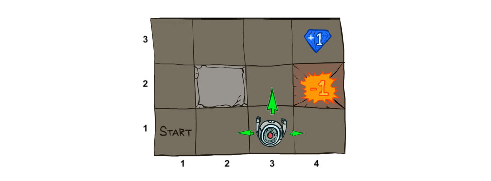
Image credit to Ketrina Yim; borrowed from Berkeley's CS188 course, with permission.
The Twist: Taking the any action only moves the agent in that direction \(80\%\) of the time, and may deviate +-90 degrees instead \(10\%\) of the time (each).
In other words, attempting to move Up will move the agent Up \(80\%\) of the time, but will, \(10\%\) of the time, move it Left, and \(10\%\) of the time, move it Right.
These noisy actions thus add probabilistic considerations into the picture, since some actions may have unintended consequences.
Hold up... that doesn't sound really realistic. What are some real-life examples that map to the notion of non-deterministic actions / consequences?
Examples:
Taking the freeway (normally the best route) during an unforeseen construction project that causes detours.
Getting a flat tire while driving a car / a robot that gets sand stuck in its wheels' actuators.
How is this problem different from Multi-Armed Bandit problems?
When the agent moves, the state (its position in the grid) changes, meaning the next decision it makes will be dependent on its previous.
How is this problem different from Classical Search?
Nondeterministic outcomes mean that we cannot generate a definitive plan / solution from some initial to some goal state.
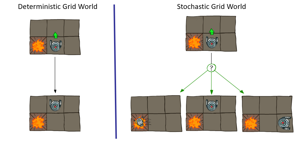
Image credit to Ketrina Yim; borrowed from Berkeley's CS188 course, with permission.
So, we'll need some different tools to approach these types of problems, starting by labeling and characterizing them!
Characterizing MDPs
Markov Decision Processes (MDPs) define stochastic search problems in which an agent attempts to maximize cumulative rewards over some (potentially infinite) time horizon.
MDPs are specified by the following properties:
States \(s \in S\): describing the environment's properties at any given time
Actions \(a \in A\): describing the actions available to the agent at any given state.
Transition Function \(T(s, a, s')\): defines the likelihood that taking action \(a\) in state \(s\) leads to the next state \(s'\): $$T(s, a, s') \Rightarrow P(s' | s, a)$$
Reward Function \(R(s, a, s')\): defines the reward obtained by taking action \(a\) from state \(s\) and landing in state \(s'\). Depending on the problem, can also be abbreviated to simply the reward associated with being in a given state: \(R(s)\)
Initial State \(S_0\): the state in which the agent begins.
[Optional] Terminal State(s): states at which the agent ceases action and cumulative rewards are "tallied".
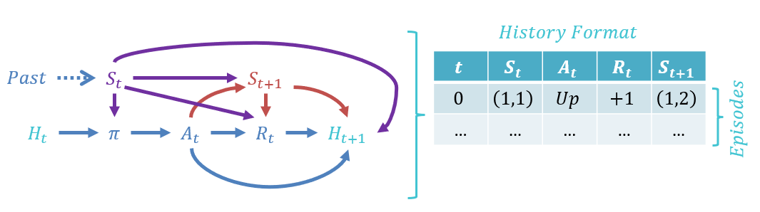
At each choice point available to the agent, its history is maintained in episodes, which are tuples of the format: $$(S_t, A_t, R_t, S_{t+1})$$ The agent's history is thus used by its policy to make choices in future time steps.
Depicted, we can see what components affect which others, and how the history might be maintained for our simple Gridworld problem:
So why "Markov" Decision Processes? Where have we heard good old Andrey Markov's name before?
Where haven't we? In Bayesian Networks, they provided the intuition behind the independence rules that led to d-separation! More akin to what we're doing now, we looked at Markov Chains / Models in which sequences of states and transitions were important.
It turns out that Markov will once again let us simplify a large portion of MDPs with a nice observation:
Intuition: Suppose we are at some maze grid cell \((2, 2)\) and are assessing the likelihood of moving Up to \((2, 3)\); does *how* we got to \((2, 2)\) influence this likelihood?
No! Once we *know* that we are at \((2, 2)\), the means by which we got there become irrelevant
The Markov Property (in general) implies that, given the present state, past and future actions and states are irrelevant for determining the current transition.
Suppose we subscript states by the times / trials at which they are encountered; the Markov Property ensures the following:
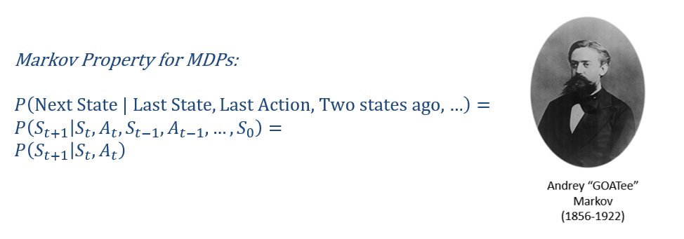
Philosophically, this is a nice result: "It doesn't matter how you got here, all that matters is what you do next."
I expect that to be printed on shirts and mugs by the time we next meet.
Functionally, the Markov Property is nice for MDPs because it allows an agent to assess action efficacies in different states without needing to account for large context-sets (like in Contextual Bandit Problems).
Let's see how that's useful next!
Policies
Because classical search fails in settings with stochastic actions, MDP agents (like MAB ones) develop a Policy \(\pi\) that maps states to actions: $$\pi: S \rightarrow A$$
Consequently, the Optimal Policy \(\pi^*\) is the one that maximizes expected, cumulative reward if obeyed.
This is slightly different than hard-and-set goals that we saw with classical search for a couple of reasons: (1) stochastic actions must be considered, and (2) rewards decide the "goals" on the fly.
Although terminal node rewards feature prominently in the optimality of policies, living rewards (which decide a "trickle") of reward to give the agent at each non-terminal step, may also influence the agent's behavior.
[Consider] What are some real circumstances that might map to the notion of a living reward?
A robotic agent that has to manage its remaining battery power and taking actions reduces it (negative living reward to minimize travel distance).
A game-playing keep-away agent that needs to avoid terminal states for as long as possible (positive living reward to maximize travel distance).
As such, we can envision how an agent with different Living Reward behaves in our gridworld example...
[Reflect] Below, the optimal policy in our Noisy Gridworld is depicted for different values of the Living Reward, \(R(s)\). Rationalize why the optimal policy attempts the actions that it does.
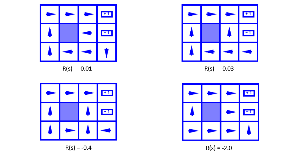
Borrowed from Berkeley's CS188 course, with permission.
Now, just how we go about *finding* these policies is the topic of another day -- more next time!