Sequences of Rewards
Last we left off, we wanted to find the mechanisms by which we could derive an optimal policy in a Markov Decision Process.
Before we do so, we need to take a step back and consider just what an optimal policy should deliver.
[Review] What is a policy's goal?
To maximize cumulative reward of the agent throughout its lifetime.
Note that by "cumulative" reward, this implies a series of decisions whose efficacy we want to maximize.
Policy Property 1: an optimal policy should maximize the received reward over a sequence of chosen actions.
This sounds fairly obvious, but what is a less obvious consequence is the following:
Suppose we have two 3-action sequences with the same, total, cumulative reward; which might we prefer and why? $$S_1 = [0, 0, 1];~~ S_2 = [1, 0, 0]$$
We would likely prefer the second action sequence because the rewards are received sooner than later; this is desirable because:
Sooner is just typically better! If you win the lottery, it's better to have the money in-hand ASAP rather than, say, the same amount just before you die! Economically, having the reward sooner means you can invest and receive a return on that investment as well.
Delayed reward is more susceptible to chance. Remember that we're dealing with stochastic search problems, so more variance (and thus, less predictability) may be found over later parts of an action sequence.
Policy Property 2: heuristically, successful policies typically prefer immediate reward to delayed, though should be able to reason over both.
Sounds reasonable; we even have an adage that expresses a (similar) sentiment: "A bird in-hand is worth two in the bush."
Although not a perfect analogy, the sentiment is that the certain option at hand can be more desirable to a risky one in the future.
So then, how do we go about encoding this preference for more immediate rewards?
We can have our agent devalue those in the future by some sort of "discounting!"
Discounting
It's a fire-sale in here! (oh... not that kind of discounting)...
Discounting is the process of devaluing future reward for the purpose of preferring more immediate, and is typically accomplished through some exponential reward decay.
The discount factor \(\gamma^k\), for some \(0 \le \gamma \le 1\) is traditionally used discount some reward that is \(k\) steps away.

Borrowed from Berkeley's CS188 course, with permission.
The notion of Utility of some sequence of actions and their corresponding rewards, denoted \(U([R_0, R_1, ...])\), can be computed as a sum of discounted rewards: $$U([R_0, R_1, R_2, ...]) = \gamma^0 * R_0 + \gamma^1 * R_1 + \gamma^2 * R_2 + ...$$
With a discount factor of \(\gamma = 0.5\), which sequence of actions with the following rewards would we prefer? $$S_1 = [3, 2, 1];~~ S_2 = [1, 2, 3]$$
To answer the above, we can simply examine the Discounted Utilities of each sequence: \begin{eqnarray} U[S_1] &=& \gamma^0 * S_1[0] + \gamma^1 * S_1[1] + \gamma^2 * S_1[2] = 1 * 3 + 0.5 * 2 + 0.25 * 1 = 4.25 \\ U[S_2] &=& \gamma^0 * S_2[0] + \gamma^1 * S_2[1] + \gamma^2 * S_2[2] = 1 * 1 + 0.5 * 2 + 0.25 * 3 = 2.75 \\ \end{eqnarray}
\(U[S_1] \gt U[S_2]\), therefore we prefer \(S_1\).
Discounting's Effect on Policy
Why is the ability to set a discount factor important for policy design? [Hint: think about what a value of \(\gamma\) that is low vs. high will change about the agent].
Several reasons:
It allows us to scale how far into the future an agent should weight some delayed reward; this allows us to make conservative vs. daring agents.
It allows an agent to reason in environments with an inifinte time horizon (at which point, \(lim_{k \rightarrow \infty} \gamma^k = 0\)).
As we'll see soon (a consequence of the point directly above), this allows some algorithms to converge where they may otherwise infinitely recurse.
Warning: the following effects of a discount factor on policy may be detrimental for maximizing cummulative reward, but can be used to shape agent behavior that conforms to different metrics of success.
To see these effects in practice, consider the following, simple "bridge-walking" scenario.
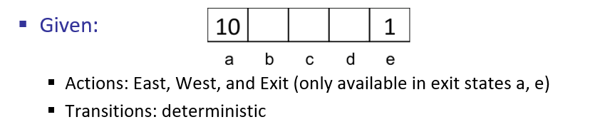
Borrowed from Berkeley's CS188 course, with permission.
For states \(b, c, d\), what action would the optimal policy \(\pi^*\) choose for discount factor \(\gamma = 1\)?
A discount factor \(\gamma = 1\) means there is *no* devaluing of future actions, so the optimal policy would favor the \(a\) terminal state: $$\pi(b) = \pi(c) = \pi(d) = \leftarrow$$
For states \(b, c, d\), what action would the optimal policy \(\pi^*\) choose for discount factor \(\gamma = 0.1\)?
A discount factor \(\gamma = 0.1\) means the agent will prefer nearer rewards, even if they are globally suboptimal, so the "optimal" policy would favor the \(a\) terminal state in states \(b,c\) but the \(e\) terminal in state \(d\): $$\pi(b) = \pi(c) = \leftarrow; \pi(d) = \rightarrow$$
Some remarks on the above:
Note that in the second case, the policy that amounts from a small discount factor \(\gamma = 0.1\) is not optimal for some infinite time horizon, but may be relevant with a small time horizon (e.g., \(T = 2\)) or large penalty for the Living Reward.
Discount factors are generally assumed / necessary for tackling MDPs with inifinite time horizons, lest it be impossible to understand the values of certain states.
How are discount factors different from living rewards?
Living rewards encode some signal from the environment whereas discount factors influence the agent's perspective of it.
So, with these goals and insights in mind, let's consider how, algorithmically, we would go about *deriving* the optimal policy.
Expectimax Search
Assumption: Before we address a harder problem later, let's begin by solving an MDP when we know the problem's states, rewards, and transitions a priori (even though these may be stochastic).
Solving a known MDP is a form of offline planning, which is an assumption we will later soften with RL techniques.
So, the input to our "solver" is to be a fully-specified MDP, and the intended output is the optimal policy, \(\pi^*\). How do we go about this?
In the past, we used Classical Search strategies to produce a plan that led from the initial to the goal state. Would these techniques be appropriate here?
No! Those planners relied on deterministic systems -- in the general MDP setting, transitions may be non-deterministic, and so plans can be easily disrupted at any stage.
As such, for inspiration, what other search strategy did we examine that didn't so much return a plan, but the best action from some state? What were its properties?
Minimax Search! It returned the best action from a given game state in an adversarial search setting. The mechanics of this were alternating min and max nodes (in a 2 player game) through which utility could be "bubbled up" from the terminal states.
As such, it seems as though *chance* is our adversary in the MDP setting.
[Brainstorm] Can we take inspiration from the above to treat the task of deriving an optimal policy (i.e., find the best action from any state such that \(\pi^*: S \rightarrow A\)) as a search problem?
Expectimax Mechanics
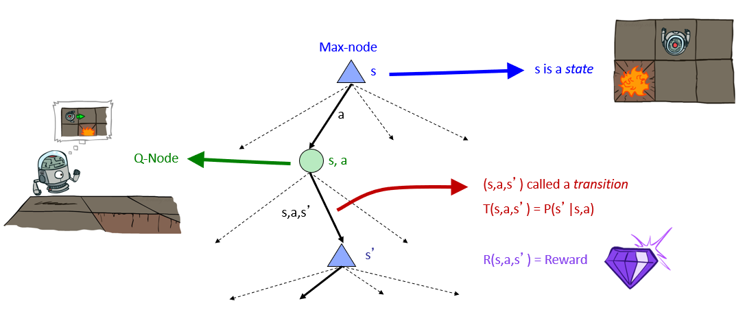
Expectimax Search is a formalization for determining the best action from a given state in stochastic search domains.
Expectimax operates by employing an expectimax tree composed of:
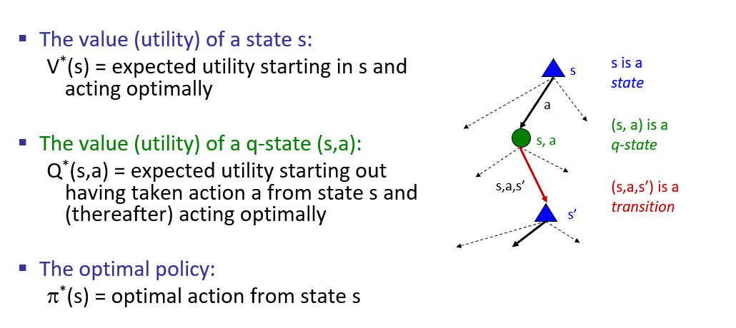
Max Nodes: representing states and have value equivalent to the maximum expected utility of its actions.
Chance / Q-Nodes: encode the transition probabilities, and are found between the tree plies connecting any 2 states.
Depicted, an expectimax tree looks like:
Borrowed from Berkeley's CS188 course, with permission.
Since reward signals in MDPs are functions of the state they were taken within \(s\), the action taken \(a\), and the state transitioned to \(s'\), they are located along the transition edges from q-states to states. Thus our notation for received rewards: $$R(s, a, s')$$
Some things to note about this fact:
Important: rewards are not collected at the states themselves, but rather, the transitions between them.
Because these transitions are mediated by q-states (chance nodes), they may be weighted by their likelihood of attainment.
\(R(s, a, s')\) is the most general representation of rewards, even if the actual reward function simply assigns values to destinations \(R(s')\) (there are some settings wherein reward may rely on source state, the action chosen, and also the destination state).
Observant readers will note, however, that to obtain these rewards for the purposes of policy-formation, we lack a stopping-condition / base-case in the event that the expectimax tree extends forever.
What tool from earlier can help us enforce such a base case and ensure that we obtain values for actions in what might be an infinite tree? How would you apply it here?
Discounting! Each ply of the expectimax tree represents another exponentiation of the discount factor soas to ensure that the lower levels of the tree more-or-less 0 out.
Depicted, this looks like:
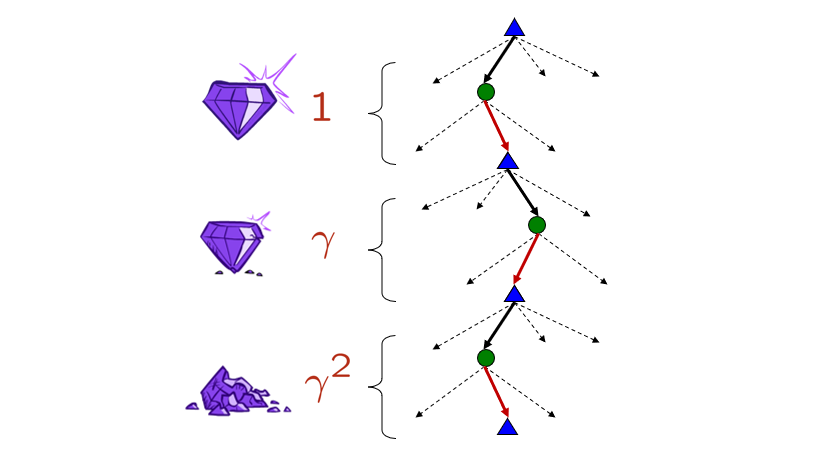
Borrowed from Berkeley's CS188 course, with permission.
So, with this new tree structure in mind, let's talk about how to actually solve an MDP by deriving the optimal policy.
Solving MDPs
To recap:
We want to find some optimal policy for an MDP (where a policy maps a state to some action).
The optimal policy maximizes utility from each state (where utility is the sum of discounted rewards).
To translate expectimax trees into policies, we should first discuss the metrics of optimality that they encode and which we want to extract.
Let's start with an abstract Expectimax tree and reason over how we would go about deducing this.
In Minimax search, how did we deduce the optimal action from a state under consideration?
Found values at some terminal states (or those at some depth-cutoff) and then bubbled-up the minimax scores to inner-nodes.
Intuition: we can attempt to do the same thing with expectimax by assigning value / utility scores to each node based on their potential for future reward.
So how do we establish these utilities / values for each node?
Borrowed from Berkeley's CS188 course, with permission.
Observation: establishing the value of any node relies on knowing the values / utilities of its children!
This observation provides recursive definitions for our targets of optimality: the values of each node in the expectimax tree.
The Bellman Equations provide recursive solutions to assess the value of each node in the expectimax tree.
Intuition: define the value of each expectimax tree node solely on the nodes below it such that if you knew the values of the children, you could easily compute the value of the parent!
We can start with definitions closest to the rewards, which are found along transitions emanating from the q-nodes.
How should the values of q-states be assessed?
A probability-weighted sum of their rewards, plus the discounted values of the states that follow.
Bellman Equation 1 - Q-State Value: the value of a q-state / q-node, denoted \(Q^*(s, a)\), for all of its transitions to states \(s'\) is: $$Q^*(s, a) = \sum_{s'} P(s' | s, a) [R(s, a, s') + \gamma V^*(s')]$$
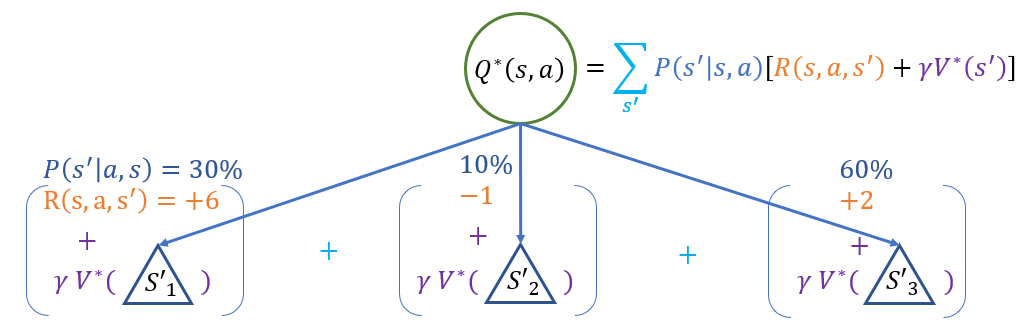
Note that the value of states to which the q-state leads (\(V^*(s')\)) assess the value of acting optimally from after the transitions.
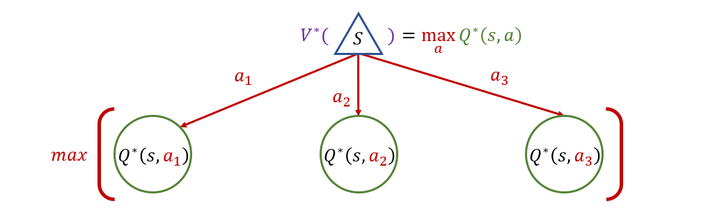
How do we assess the values of states, *remembering* that at states, the agent has the choice of action and is not subject to chance (that's encoded in the q-states)?
The utility of a state node is simply the maximum of its child q-states!
Bellman Equation 2 - State Value: the value of a state, denoted \(V^*(s)\), is simply the maximum of its child q-state values, if it has children; 0 otherwise, as a recursive base case: $$V^*(s) = \begin{cases}max_a Q^*(s, a) & \text{if}~\exists~T(s,a,s')\\0 & \text{otherwise} \end{cases}$$
Combining these two equations yields the full, recursive definition for node values: $$V^*(s) = max_a \sum_{s'} P(s' | s, a) [R(s, a, s') + \gamma V^*(s')]$$
Notes on the above:
To distinguish the two values:
\(V^*(s)\) = "what is the utility of \(s\) if the agent acts optimally from here on out"
\(Q^*(s, a)\) = "what is the utility if the agent acts optimally *after committing to* action \(a\) from state \(s\)"
Since these definitions are recursive, the base case is that the value of terminal states / leaves in the tree is, intuitively, 0.
Note that the discount factor \(\gamma\) is multiplied by each subsequent state-value, giving it the desired exponential-decay behavior.
Now, returning to the original task, how do we use the values of each node to form the optimal policy?
For each state, choose the action that simply maximizes the utility if we commit to it! In other words, maximize the q-value!
As a consequence of the Bellman Equations, the optimal policy \(\pi^*(s)\) maps each state \(s\) to the action maximizing its q-value: $$\pi^*(s) = argmax_a Q^*(s, a)$$
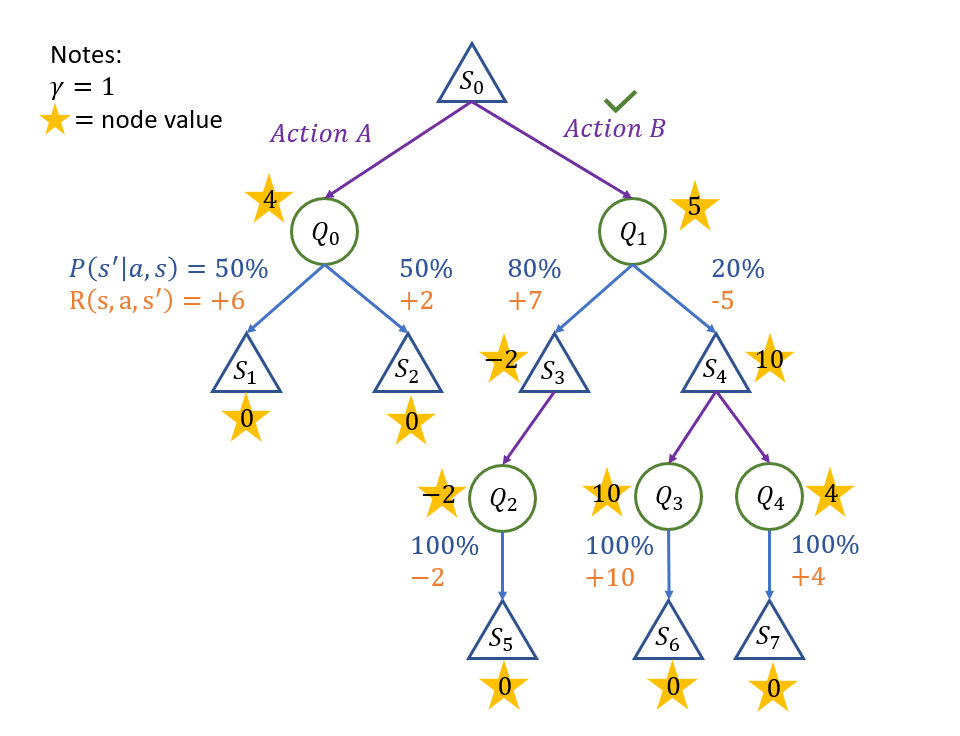
Example
Whew! That was a lot of words, why don't we see an example so we won't be intimidated by scary equations?
How do we go about determining which is the best action from state \(S_0\) in the following expectimax tree? (assume a discount factor \(\gamma = 1\), for simplicity).
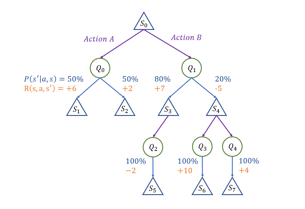
Starting with the basics: we know that the values of all leaf nodes will be (by default) 0, since rewards are accumulated on transitions alone.
So, already, we have the values of states \(1, 2, 5, 6, 7\), yay!
Let's then start by "bubbling" rewards up in the left subtree:
\begin{eqnarray} Q^*(S_0, A) &=& \sum_{s'} P(s' | s, a) [R(s, a, s') + \gamma V^*(s')] \\ &=& P(S_1 | S_0, A) [R(S_0, A, S_1) + V^*(S_1)] + P(S_2 | S_0, A) [R(S_0, A, S_2) + V^*(S_2)] \\ &=& 0.5 * [6 + 0] + 0.5 * [2 + 0] \\ &=& 4 \end{eqnarray}
Since \(Q_2, Q_3, Q_4\) all have deterministic transitions, we see that their values are the same as their transition rewards, so can complete those easily.
The same ease follows for \(S_3\) who, with only a single action available, attains that value as well.
\(S_4\) is about as simple, but we remember that: $$V^*(S_4) = max_a Q^*(S_4, a) = max(10, 4) = 10$$
Finally, the trickiest of them all, \(Q_1\), due to having the values of its children \(S_3, S_4\), can be computed immediately:
\begin{eqnarray} Q^*(S_0, B) &=& \sum_{s'} P(s' | s, a) [R(s, a, s') + \gamma V^*(s')] \\ &=& P(S_3 | S_0, B) [R(S_0, B, S_3) + V^*(S_3)] + P(S_4 | S_0, B) [R(S_0, B, S_4) + V^*(S_4)] \\ &=& 0.8 * [7 - 2] + 0.2 * [-5 + 10] \\ &=& 5 \end{eqnarray}
Finally, we develop our policy for each state in the Expectimax tree, but just to intimate, in particular, for the root \(S_0\): $$\pi^*(S_0) = argmax_a Q^*(S_0, a) = B$$
The final, completed tree: