Value Iteration

In the previous lecture, we saw Expectimax Trees as ways of assessing state utility / values through a recursive definition of the Bellman Equations.

However, we should assess some practical concerns with using "raw" expectimax trees for this purpose.

[Reflect] What are some issues with solving the Bellman Equations using raw expectimax trees like we saw in the last lecture?

tl;dr, naive expectimax is doing too much work!

Just to highlight the couple points you likely came up with:

Problem 1: In the expectimax tree, repeated states may often occur -- what shall we do?

Memoize values once they're computed!

Seems simple enough -- we don't want to recompute anything that we've already computed, basic!

We can imagine that this happens a lot: in the Noisy Gridworld, our Expectimax tree would represent actions of moving back and forth from the same spot.

More serious is the following:

Problem 2: Even with discount factors, the expectimax trees may extend forever! How can our algorithm know "when to stop?" [Hint: think about what we did to tackle depth-first-search's potentially infinite recursion within the confines of classical search].

Perform some sort of depth-limited computation, with increasing depths until the values have converged!

Value Iteration

Value Iteration is a strategy for finding $V^*(s)~\forall~s$ in an MDP, which can then be used to find $\pi^*$.

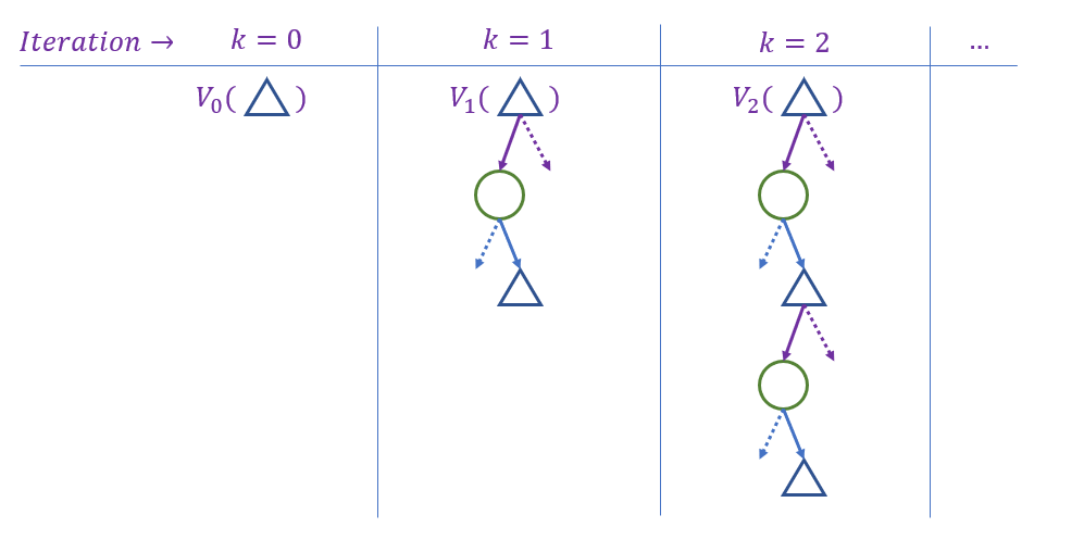
Value Iteration accomplishes this by finding Time limited values, $V_k(s)$ that compute the value of state $s$ equivalent to what an expectimax tree of state-depth $k$ would return.

Intuition: starting with the base case which $k = 0 \Rightarrow V_0(s) = 0$, build values up ply-by-ply. Continue until $V_k(s) \approx V^*(s)$.

What sort of algorithmic paradigm captures the case of starting with small subproblems and then building on top of those to reach larger, more complex ones?

Bottom-up Dynamic Programming!

Hey! So that Algorithms stuff wasn't useless after all? Fancy that!

Using bottom-up DP gracefully solves the issue of repeated states, but how do we avoid infinite trees?

Value iteration operates as follows:

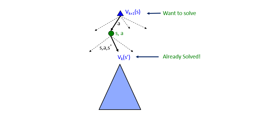
Starting with a vector of state values $V_k(s)$, compute one ply of expectimax from each state by the Bellman Update Rule: $$V_{k+1}(s) \leftarrow max_a \sum_{s'} P(s'|s, a) [R(s, a, s') + \gamma V_k(s')]$$

In words, the Bellman Equations characterize / describe the optimal values, but to actually attain them, we can use Value Iteration as a means of computing them.

Borrowed from Berkeley's CS188 course, with permission.

Two conceptual followup questions:

How will we know when $k$ is large enough to stop performing the Bellman Updates?

When the values converge, i.e., between no two iterations are there any substantial changes to the values. $$V_k(s) \approx V_{k-1}(s)~\forall~s$$

In the Noisy Gridworld domain, value iteration looks like the following:

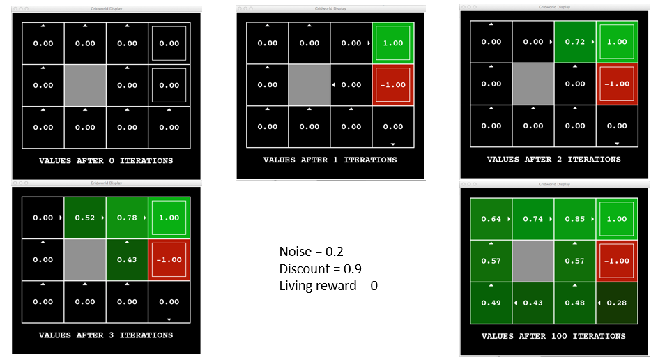
Borrowed from Berkeley's CS188 course, with permission.

Let's take a look at a more hands-on example!

Example

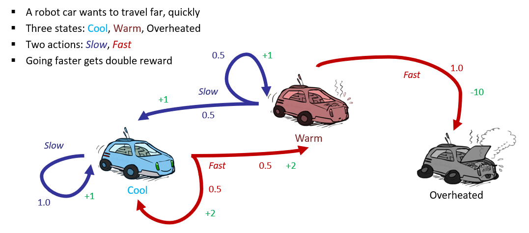
Borrowed from Berkeley's CS188 course, with permission.

If we were to depict the expectimax tree associated with this example, and then highlight the time-limited values of each car state (i.e., cool, hot, overheated), we would see the following for 5 plies:

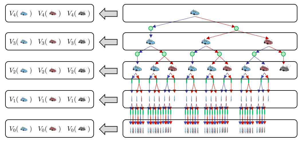
Borrowed from Berkeley's CS188 course, with permission.

For the racing example, compute the first few plies of value-iteration (i.e., compute $V_2(s)~\forall~s$) assuming $\gamma = 1$.

Finding $V_0(s)~\forall~s$:

Easy, this is our base case, so $V_0(s) = 0~\forall~s$. Recall that this would be akin to computing the value for a state in a time-limited expectimax tree with no time left!

Finding $V_1(cool)$:

We'll need to first find Q*, i.e., the max over all actions $a \in \{fast, slow\}$ of their probability weighted transitions starting in the cool state.

\begin{eqnarray} Q_1(cool, slow) &=& \sum_s' P(s'|s,a)[R(s,a,s') + \gamma V_0(s')] \\ &=& P(cool|cool, slow) R(cool, slow, cool) \\ &=& 1 * 1 \\ &=& 1 \\ Q_1(cool, fast) &=& P(cool|cool, fast) * R(cool, fast, cool) + P(warm|cool, fast) * R(cool, fast, warm) \\ &=& 0.5 * 2 + 0.5 * 2 \\ &=& 2 \\ \end{eqnarray}

Plainly, then, $max_a Q_1(cool, a) = 2$, so for our update we have:

$$V_1(cool) \leftarrow max_a Q_1(cool, a) = 2$$

Finding $V_1(warm)$:

Similar to what we did above, but now for the warm state, we have:

\begin{eqnarray} Q_1(warm, slow) &=& \sum_s' P(s'|s,a)[R(s,a,s') + \gamma V_0(s')] \\ &=& P(cool|warm, slow) R(warm, slow, cool) + P(warm|warm, slow) R(warm, slow, warm) \\ &=& 0.5 * 1 + 0.5 * 1 \\ &=& 1 \\ Q_1(warm, fast) &=& P(overheated|warm, fast) * R(warm, fast, overheated) \\ &=& 1 * (-10) \\ &=& -10 \\ \end{eqnarray}

Got it: don't go fast when warm! So, $max_a Q_1(warm, a) = 1$, so for our update we have:

$$V_1(warm) \leftarrow max_a Q_1(warm, a) = 1$$

Finding $V_1(overheated)$:

This one's easy (finally) -- once we're overheated, we're doneskis, this is a terminal state:

$$V_k(overheated) \leftarrow 0~\forall~k$$

Finding $V_2(cool)$:

Now, comes the harder part since we're not leaning on a base case of $V_0(cool) = 0$, we'll have to incorporate the values of a deeper expectimax tree that instead knows the values of the ply beneath it:

\begin{eqnarray} Q_2(cool, slow) &=& \sum_s' P(s'|s,a)[R(s,a,s') + \gamma V_1(s')] \\ &=& P(cool|cool, slow) [R(cool, slow, cool) + 1 * V_1(cool)] \\ &=& 1 * [1 + 2] \\ &=& 3 \\ Q_2(cool, fast) &=& P(cool|cool, fast) [R(cool, fast, cool) + 1 * V_1(cool)] \\ &+& P(warm|cool, fast) [R(cool, fast, warm) + 1 * V_1(warm)] \\ &=& 0.5[2 + 2] + 0.5[2 + 1] \\ &=& 3.5 \\ \end{eqnarray}

Once more, $max_a Q_2(cool, a) = 3.5$, so:

$$V_2(cool) \leftarrow max_a Q_2(cool, a) = 3.5$$

Finding $V_2(warm)$:

Left as an exercise, but it's 2.5.

To summarize:

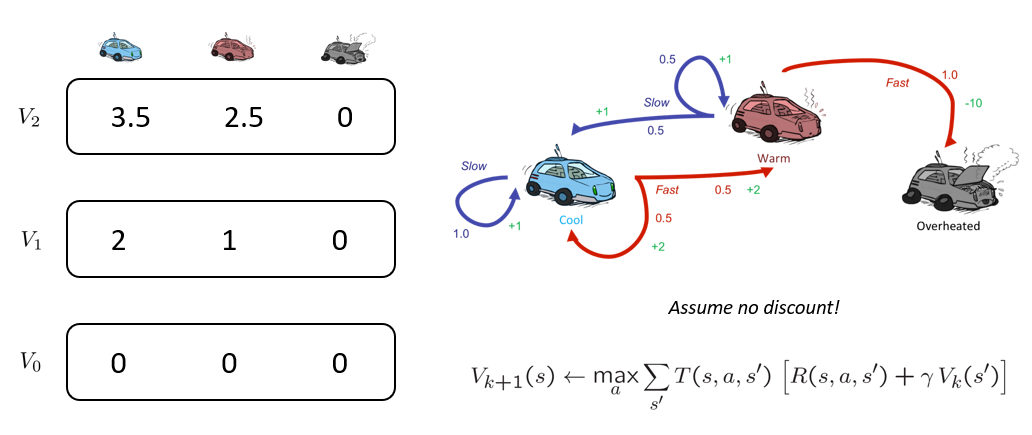
Borrowed from Berkeley's CS188 course, with permission.

Convergence Guarantees

So why does this work, and how do we guarantee that it will?

Theorem: $lim_{k \rightarrow \infty} V_k(s) = V^*(s)$.

We can sketch a proof as to why:

Case 1: (easy case) the expectimax tree that we're iteratively deepening actually does have a depth-limit, so the values discovered by iteratively deepening are the true ones.
Case 2: there is no depth limit to the tree, but since we are applying an exponentially increasing discount factor, later plies 0 out in expectation.

Neat result! ...but can we do better?

Policy Iteration

Before we sell the farm on value iteration, we should answer a couple evaluative questions:

[Reflect] Determine some points of weakness for value iteration.

The biggest weaknesses:

Learning values $V(s)$, for most applications, is good only in support of finding the optimal policy, which will converge to the best action at each state much earlier than before the values converge.
The best action at each state is almost always the same between iterations (so wasted effort recomputing the max $Q_k(s, a)$).
It is not computationally attractive, requiring $O(|S|^2 * |A|)$ computations for *each* iteration.

So, examining the above complaints, we make two remarks: (1) we learn values in pursuit of finding an optimal policy, and (2) we still have (in these offline MDP solvers) knowledge of the transitions and rewards. How can we improve on value iteration?

Start with *some* policy (any one will do), and then tweak it to become the optimal policy!

This new approach is called Policy Iteration and proceeds in several steps:

Fixing a Policy $\pi_i$: fix the behavior of some (possibly, originally suboptimal) policy -- it has some behavior that it will take for all states.
Policy Evaluation $V^{\pi_i}$: determine the value / utility of each state according to that fixed policy.
Policy Improvement $\pi_i \leftarrow \pi_{i+1}$: tweak the previous policy version to be more optimal!

Policy Evaluation

To see why this new approach is attractive, consider the two expectimax-like trees that we are evaluating for each of value- vs. policy-iteration:

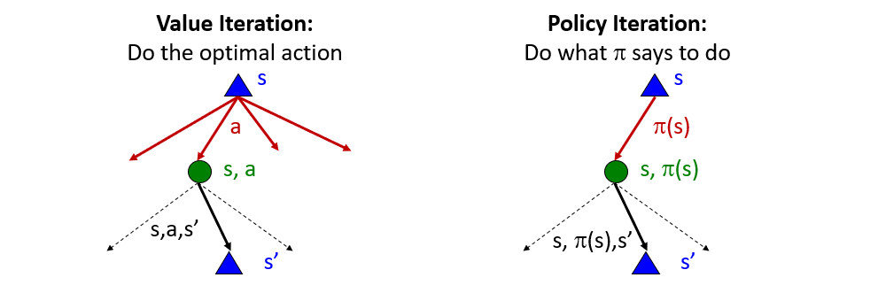
Borrowed from Berkeley's CS188 course, with permission.

What's nice about this new "fixed policy expectimax" tree on the right, and how does it relate to some Algorithms topics on Search?

It only has 1 action at each state to consider, meaning we no longer have to maximize over multiple possible actions -- the branching factor of the resulting expectimax tree is reduced!

Utilizing this "skinnier" tree gives us some computational improvements, and all that it requires is that we consider the value associated with each state given some fixed policy.

Establishing fixed policy values defines the utility of a state $s$ under some policy $\pi$ such that: $$V^{\pi}(s) = \text{Discounted rewards starting in s and acting according to policy}$$

Once more, we can use the Bellman equations to characterize what this new quantity recursively:

The Bellman Equations for these policy-specific state values can be used to characterize (in the same way as before) the value recursively: $$V^{\pi}(s) = \sum_{s'} P(s'|s, \pi(s)) [R(s, \pi(s), s') + \gamma V^{\pi}(s')]$$

Before, we noted that the Bellman Equations described / defined some target estimation, but the way we actually computed it was through an iterative process; the same will be true for us now!

Policy Evaluation provides an iterative mechanic for computing the fixed policy values, borrowing from the tools of value iteration such that we perform the following time-limited policy values (for max depth $k$) until values converge: $$V^{\pi}_{k+1} \leftarrow \sum_s' P(s'|s, \pi(s)) [R(s, \pi(s), s') + \gamma V^{\pi}_k(s')]$$

This will, for the given policy $\pi$, converge to the policy-specific utilities of each state, and with much better complexity of $O(|S|^2)$.

However, this is only useful insofar as it "grades" the quality of a policy in any given state; reasonably, you must ask: how do we then get or evolve a better policy?

Policy Improvement

To reiterate: we are still doing offline MDP planning, meaning we know the transition probabilities and rewards at each state!

With that said, we can, for any given state, perform a one-ply lookahead at all possible actions (not just the ones that a given policy has chosen) to determine what the best action is for a state based on the current policy's fixed values.

Policy Extraction chooses a new, maximal action in terms of the previous policy's, $\pi_i$, state values $V^{\pi_i}$, such that a *new* policy $\pi_{i+1}$ can be extracted via: $$\pi_{i+1}(s) = argmax_a Q^{\pi_i}(s, a) = argmax_a \sum_s' P(s'|a,s)[R(s, a, s') + \gamma V^{\pi_i}(s')]$$

Note: the above is crucially different because $argmax_a$ examines the best of *all possible* actions from some state $s$, not just the one that is being chosen by the current policy.

In words, policy "version 2.0" (then 3.0, then 4.0, etc.) are going to use the previous policy's utilities to then find a new, better policy, even if that means changing the policy's actions 1 state at a time.

Policy Iteration

Fun fact: the abbreviation for "Policy Iteration" is "PI", the greek letter associated with the policy (coincidence? I think not...).

In other news, let's recap:

Policy Evaluation allows us to score the utility of each state under some fixed policy.
Policy Improvement allows us to perform a one-step lookahead at each state and determine if a better policy exists, though still based on the previous policy's values (which have been computed efficiently.)

So, let's put those two together to complete our policy iteration approach to finding an optimal policy:

Step 1: compute $V^{\pi_i}(s)~\forall~s$ via policy evaluation.
Step 2: compute $\pi_{i+1}(s)~\forall~s$ via policy improvement.
Step 3: repeat above until $\pi_i(s) = \pi_{i+1}(s)$

Example

Reconsider the "Bridge" example that we saw with our introduction to discounting, and how policy iteration can help!

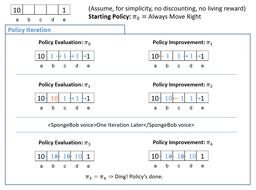
Obviously, the above is a very simplified example of policy iteration given that it lacks: discounting, stochasticity, and living rewards, but you get the idea of the policy iteration mechanics now!

Review

A review section *within* the lecture?

Let's take a step back at what we've seen today:

Value- and policy-iteration do the same thing, but with different approaches. Policy iteration is typically much faster because of the problems with value iteration (highlighted at the start of this section) that it addresses.
Both of these approaches employ dynamic programming in concert with the Bellman Equations to efficiently compute discounted future rewards.
Moreover, if policy iteration *begins with* a decent policy, then it will not need many updates during the policy improvement stage and can converge even more quickly.

Crucially: each of these approaches is being done for offline MDP solving!

Next time, as you might've guessed, we look at the harder (but more interesting) case: online MDPs!