Reinforcement Learning - Perspective
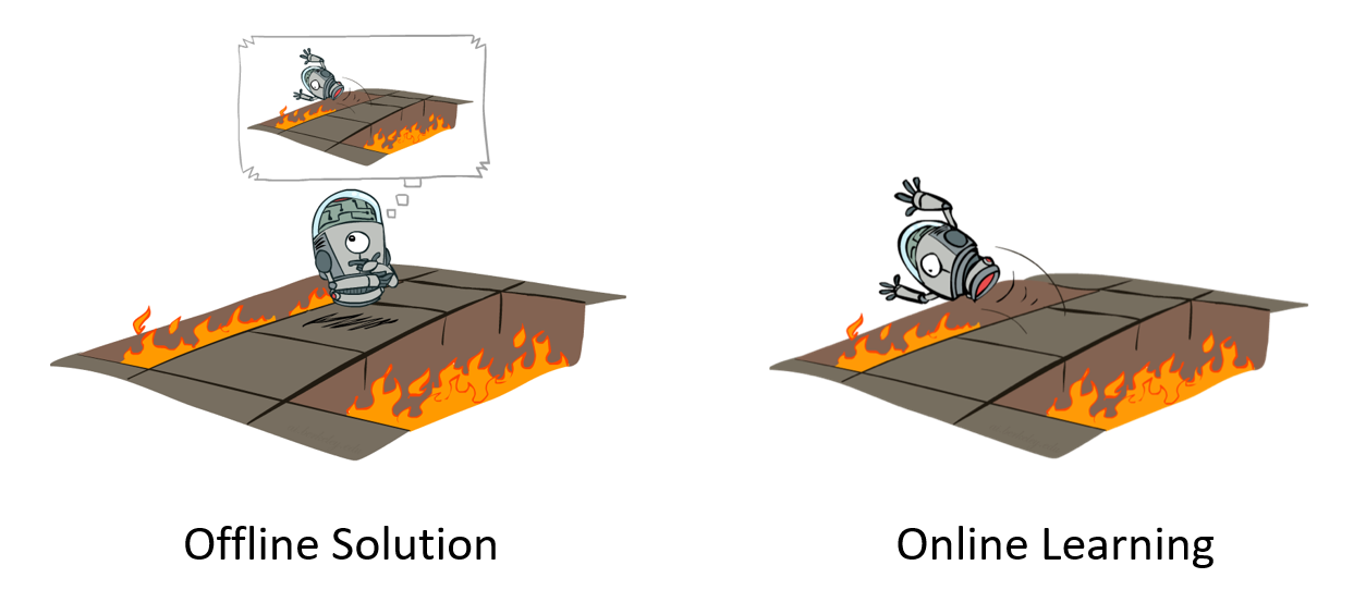
Thus far, we've been solving MDPs in the offline domain wherein all facets of the environment are known and available to the agent.
Policy extraction in these settings has been more of a computational challenge than a practical one, since the pieces are all there, it's just up to us to be clever putting them together.
However, these settings rely on the strong assumption that we even have all of the information about the environment to start -- we should be able to have agents that develop optimal policies on their own!
Examining these offline domains was not useless, as it gifted us the "sunny skies" targets of the Bellman Equations, value functions, q-value functions, and how to extract the optimal policy from these.
Now, let's look at a (perhaps more interesting, but certainly) more general specification...
New Problem Specification: Partially Specified MDPs wherein transitions and rewards are initially unknown to the agent at the start. The goal is the same: maximize cumulative rewards.
Offline MDP solving is a planning problem whereas Online MDP solving is a reinforcement learning problem.
Borrowed from Berkeley's CS188 course, with permission.
Let's start with some assumptions about this new domain of MDPs:
The environment is still an MDP, but we do not possess the transition function \(T(s, a, s')\) nor the reward function \(R(s, a, s')\).
These functions *can* be learned by exploring the environment, taking actions and learning their results in the form of episodes \((s, a, s', r)\).
The agent is assumed to be capable of repeat trips through the environment, starting at the initial state, hitting a terminal, and restarting with knowledge gained from the previous iterations.
Our objectives in these partially-specified MDPs are largely twofold:
How do we evaluate / score states of an existing policy in a partially-specified MDP?
How can an agent extract the optimal policy from them?
Approaches
There is much diversity in how to approach these goals, but we should be comfortable with some labels for these different approaches.
There are two classes of agency for RL learners:
Passive RL: the learner takes notes on being instructed on how to act by some fixed policy; they're "along for the ride."
Active RL: the learner has full agency and can choose whatever actions it wants to take in the environment.
Note: in both of these cases, the agent is still acting and operating in the environment, just like with the MAB problem!
Suppose you are learning a fighting game and are told by a friend to try out some combination of moves (passive RL); you get to see the effects of that policy, but will not learn new combos until you experiment yourself (active RL).
Just what the agent learns along the way (in either case) is a consequence of their objective.
The fruits of RL learning are generally divided into two camps:
Model-Based Learning: the agent tries to (in some way) reconstruct the underlying MDP, and then solves it using the previously discussed methods.
Model-Free Learning: underlying MDP be damned! The agent just wants to learn the best policy (i.e., best action given any state).
Model-Based approaches can be more interpretable and can incorporate background information, but may waste effort exploring the environment where a more performance-focused model-free agent may excel.
Let's look at some of these techniques now!
Model-Based Learning
Let's begin with our first objective: to find an empirical / sample-based means of evaluating some policy.
Model-Based Learning techniques proceed in 2 general steps:
Learn an approximate model of the MDP based on experience (active RL), some demonstration from an expert / teacher (passive RL), and even an external dataset (supervised learning).
Use that approximation of the MDP to do value / policy iteration.

Basically, Model-Based approaches try to make a DIY MDP and then use the techniques we discussed last lecture!
How would we, naively, go about this task if our agent were attempting to learn in the active RL setting?
Take a bunch of random actions in the environment, record the episodes \((s, a, s', r)\), and then estimate the transitions and reward functions from these.
The benefits of model-based approaches are still evolving, and include:
The ability to learn more complex *causal* relationships between variables in the system and state, which can be useful for planning if distinguished from observation.
The ability to transport experiences learned in one environment to other ones in which only some facets are different.
What's the main issue with Model-Based approaches?
Mainly: it would take forever to get accurate estimates for the transitions and rewards for large state-action spaces, especially if some states / rewards are distant from the initial state. Meanwhile, the optimal / good policy could likely be found in a fraction of the time.
NB., the field moved away from model-based approaches with the deep-learning fervor, but some techniques have started to come back into vogue, especially now that the limits of DL are being felt, and transportability of learned experiences remains a problem!
As such, we won't have a lot to say about model-based approaches herein, since most fail to compare to the state-of-the-art, but keep your eye on this paradigm of techniques as the field progresses.
Model-Free Learning
Model-Free Learning is a class of techniques for learning optimal policies to partially-specified MDPs by attempting to estimate state values, and then constructing a policy from those estimates.
There are a variety of ways to do this that we'll see, but in the online, partially-specified MDP domain, we still have a couple of tasks:
Policy Evaluation: given some policy \(\pi\), determine the expected value from following it.
Policy Improvement: given some starting policy \(\pi_k\), find a "next" / "better" policy \(\pi_{k+1}\).
The biggest challenge of the above: since we're sampling states, transitions, and rewards all at once, our estimates for values will be shifting with each episode!
As such, we have a few tasks ahead of us:
What tools allow us to keep a "moving average" of witnessed values, even in spite of nondeterministic transitions / rewards?
How can we perform policy evaluation using these tools?
How can we perform policy improvement, and how will our evaluative tools come into the picture?
Exponential Moving Averages (EMA)
In many situations, we are faced with noisy trends that fluctuate over time, but wherein we want some estimate of averages within time-adjacent windows.
What are some examples of such data / trends?
Stock prices that are volatile in a give week, but relatively constant within the week / month.
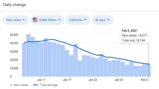
COVID-19 infection rates, as 7-day averages are reported.
Weather patterns in regions, though individual days fluctuate.
Note that from a purely data-perspective, getting these "rolling-averages" presents something of a challenge because it demands that we:
Downweight samples that were collected early because they matter less to estimation of the current trend's average.
Don't downweight *too* much because then the rolling average will be overly sensitive to the fluctuations of recent samples.
There are many techniques for managing the above, and we'll look at one of the more useful in the context of our current endeavor with online RL.
Exponential Moving Averages (EMA) provide a means (pun intended) of estimating "rolling-averages" over time in which more recently collected samples are weighted heavier than older ones.
A common format of the EMA is to define some weighting parameter \(\alpha \in [0,1]\) defining the proportion with which each new sample updates the current estimate of the rolling average such that: $$\text{new_estimate} = (1 - \alpha) * \text{old_estimate} + \alpha * \text{sample}$$
Consider some set of samples and two EMA estimates with the following choices of \(\alpha\):
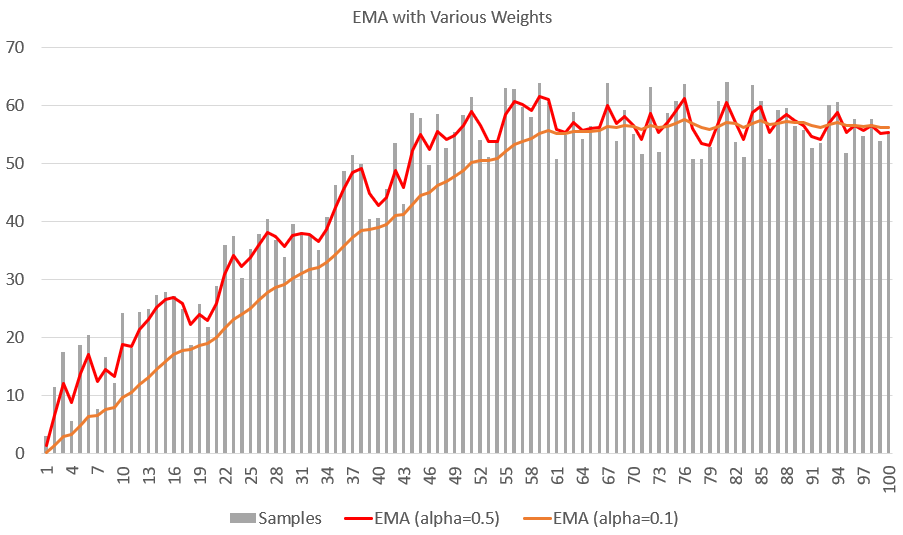
Notes on the above:
The EMA estimates at each time step (X-axis) are the estimated rolling average up until that step.
Note how the EMA estimate with a higher value of \(\alpha=0.5\) is more sensitive to the individual perturbations of the samples, but those of the smaller value of \(alpha=0.1\) are more "stubborn" and cling to the past samples, resulting in a smoother estimate that's less sensitive.
Note that this is "exponential" because up until time \(t\), each sample in the past gets discounted by a factor of \((1 - \alpha)\) such that the oldest is discounted by \((1 - \alpha)^t\).
So... how does this help our pursuit in online RL?
Temporal Difference Learning (TDL)
Temporal Difference Learning (TDL) is a model-free technique for performing passive, online, reinforcement learning for policy evaluation in a partially-specified MDP in which EMAs of state values are maintained and then updated with every episode.
Recall: passive policy evaluation = assessing the quality of a fixed policy.
Intuition: Since we're attempting to perform policy evaluation, we can use our policy iteration update rule as a roadmap in this endeavor: $$V^{\pi}_{k+1}(s) \leftarrow \sum_{s'} P(s'|s, \pi(s)) [R(s, \pi(s), s') + \gamma V^{\pi}_k(s')]$$
If we stare at this update rule long enough, maybe squinting a little, tilting our heads a bit, we can see it for what it really is: a weighted average!
In particular, what we have is, with many many samples taken, a formula of the format: $$V^{\pi}_{k+1}(s) \leftarrow \sum_{s'} \text{Chance of s'} * \text{Sample of reward and value onward from s'}$$
Here, the notion of a sample, as we might encounter while operating in our environment is of the format: $$sample = R(s, \pi(s), s') + \gamma V^{\pi}(s')$$
The temporal difference update rule for fixed policy \(\pi\) and learning rate \(\alpha\) is a type of EMA to update the value of a state given a sample collected online: \begin{eqnarray} sample &=& R(s, \pi(s), s') + \gamma V^{\pi}(s') \\ V^{\pi}(s) &\leftarrow& \text{Current value estimate} + \text{New sample adjustment} \\ &=& (1 - \alpha) V^{\pi}(s) + \alpha * sample \\ &=& V^{\pi}(s) + \alpha (sample - V^{\pi}(s)) \\ \end{eqnarray}
If our agent is trying to learn some stable, but unknown, value function \(V^{\pi}(s)\), why are we using an EMA?
Because \(V^{\pi}(s)\) is dependent on the values of other states \(V^{\pi}(s')\), which won't be accurate at the start! As such, we'll keep updating our estimate as more samples are collected, and thus *all* state values more accurately estimated.
The learning rate \(\alpha\) thus prevents the value estimates from thrashing as they iteratively improve in their accuracy. However, if we pick a learning rate that is too high or too low, the value estimates may not converge.
Inspired by one of our Action Selection Rules with the MAB algorithms, what may be a good strategy for settings of \(\alpha\)?
Once again, perform some sort of simulated annealing with a high value for \(\alpha\) early in the learning process, and then attenuating it when the agent becomes more experienced.
Let's look at an example and then make some remarks:
Suppose we have some existing knowledge of the following small gridworld model in which the far-right terminal state has a reward of 16. With the initial state \(B\), \(\gamma = 1\), \(\alpha = 0.5\), and \(\pi(s) = \text{Right}\), trace a single execution of TDL.
Note, the following example begins after the following episodes have been recorded: ((0,1), R, (1,1), +0), ((1,1), R, (2,1), +0),
((2,1), Exit, Terminal, +16)
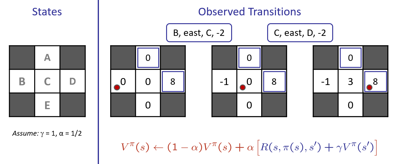
Borrowed from Berkeley's CS188 course, with permission.
Things to note from the above:
With another iteration, the value estimate for \(B\) would become positive, as the values of each state are propagated backward.
These values are inherently noisy at first, but will converge through repeated samples.
Problems with TDL
Although TDL is nice for evaluating existing policies and learning about the environment through passive RL, we might have some issues performing policy improvement using it.
Recall that to find the optimal policy, we require information about the Q-values: $$\pi^*(s) = argmax_a~Q(s, a)$$
Why does this definition of the optimal policy present a challenge for temporal-difference learning?
What we *have* through TDL are merely samples of \(Q(s, \pi(s))\), which do not necessarily explore all of the *available* actions at a given state, but merely, the ones selected by the policy.
As such, while TDL is useful for policy evaluation, we need some other tools to actually derive the optimal policy in partially-specified MDPs.
Why is it still useful to have a means of policy evaluation, even if it cannot be used to find the optimal policy?
If we have different tweaks of policies, e.g., with different living rewards, discount factors, etc., it allows us to evaluate and compare their performances.
Let's tackle finding the optimal policy given some partial-MDP specification next!
Q-Learning
Since TDL gives us a handle on policy evaluation, but not formation / improvement, we have to reflect on our desire to craft the optimal policy from optimal q-values.
In order to empirically measure these q-values, we can once again turn to the Bellman Equations that led to our value-iteration update rule:
With value iteration, we had:
Base Case: \(V_0(s) = 0\) for the expectimax tree with 0 steps left.
Recursive Case: Given \(V_k\), we can calculate \(V_{k+1}\) via the Bellman Update rule: $$V_{k+1}(s) \leftarrow max_a \sum_{s'} P(s'|s, a) [R(s, a, s') + \gamma~V_k(s')]$$
Reformatting the above (simple substitution), we can instead phrase this update rule in terms of q-values:
The Q-Iteration Update Rule is a rearranging of the value-iteration update such that: \begin{eqnarray} Q_{k+1}(s, a) &\leftarrow& \sum_{s'} P(s'|s, a) [R(s, a, s') + \gamma~max_{a' \in A(s')}~Q_k(s', a')] \\ &=& \text{Average reward of samples from acting optimally after choosing a} \end{eqnarray}
What's the problem with the Q-Iteration Update Rule specified above in online, partially-specified MDPs?
It still relies on knowing the transitions and rewards, so we'll lean on the intuitions behind Temporal Difference Learning and turn this into an empirical sampling rule.
Q-Learning
Q-Learning is a procedure for computing q-value iteration in an online, active MDP task.
Q-learning updates our current knowledge of q-values as the agent is operating in the environment.
Its steps are the same as TDL but for Q-values, as follows:
The q-learning update rule, for learning rate \(\alpha\) is specified as: \begin{eqnarray} sample &=& R(s, a, s') + \gamma~max_{a' \in A(s')}~Q(s', a') \\ Q(s, a) &\leftarrow& (1 - \alpha) Q(s, a) + \alpha * sample \\ &=& Q(s, a) + \alpha (sample - Q(s, a)) \\ &=& \text{Old q-state estimate} + \text{Sample nudge} \end{eqnarray}
What purpose does the \(max_{a'}\) have in the q-learning update rule?
It ensures that only the best action from the next state is used to inform its value from the previous!
This approach will thus maintain a tabular structure of q-values for each action taken in each state, with a record-keeping structure akin to the following:
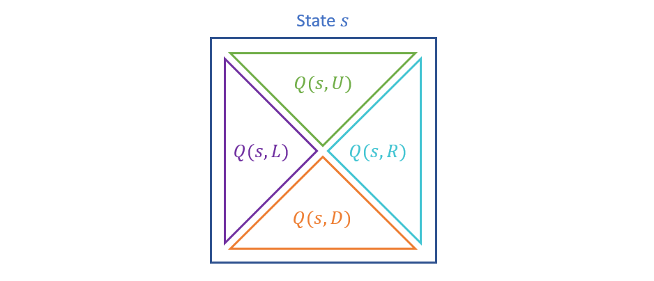
In the original gridworld formulation, this appears like the following:
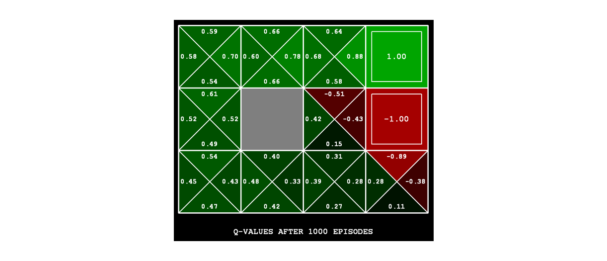
Borrowed from Berkeley's CS188 course, with permission.
Some notes on the above:
In each state, we are separately tracking the value of each action, which means we need many samples with adequate exploration to converge to the optimal policy. Thus, the same tools we used in the MAB setting to help with the exploration vs. exploitation tradeoff will again be appropriate.
Once more, we need to ensure that the learning rate is attenuated as the agent learns.
Example
Consider the following example with q-value estimates shown in the gridworld, and the agent takes the action \(R\) from state \(s\) and ends up in state \(s'\) (with its associated q-value estimates shown). Find the updates to any q-values in state \(s\) wtih \(\gamma = 1.0, \alpha = 0.1\).
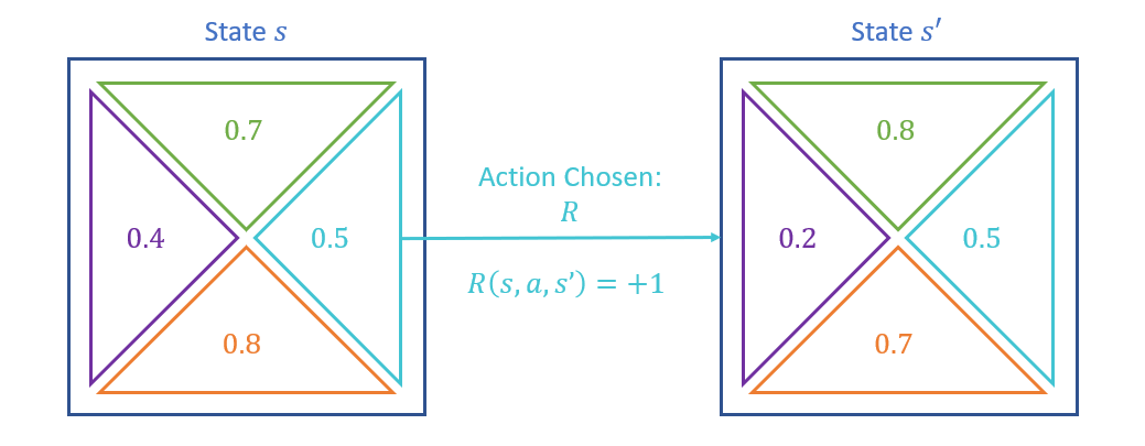
We'll start by finding the sample value here, which is defined as: \begin{eqnarray} sample &=& R(s, a, s') + \gamma~max_{a' \in A(s')}~Q(s', a') \\ &=& 1 + 1.0 * 0.8 \\ &=& 1.8 \end{eqnarray}
Next, we update the previous q-value from \(s\) and the action \(R\): \begin{eqnarray} Q(s, R) &\leftarrow& Q(s, R) + \alpha * (sample - Q(s, R)) \\ &=& 0.5 + 0.1 * (1.8 - 0.5) \\ &=& 0.63 \end{eqnarray}
Note how the update in the example above is based off the future reward from \(s'\) acting optimally, i.e., moving UP from \(s'\), *even if the agent doesn't actually move up from \(s'\) next.*
In general, even if the agent acts suboptimally during exploration, the q-values will converge due to the \(max_a'\) as part of the sample formulation. This is known as off-policy learning wherein learning can happen on actions that are not even taken by the agent.
At this point, in lecture, we'll look at some demos of q-learning!
Whew! I know that's quite a bit to digest. Luckily, next time, we'll get some practice with all of the above, and then see some ways to improve beyond the basics of q-learning!