Approximate Q-Learning

Let's think about an important issue with the type of Q-Learning we've been doing thus far, motivated by some questions.

What data structure have we been using to store / update q-values for an online q-learner? What's stored in this DS?

We've just been using a table, storing the q-values for all state-action combos, i.e., $Q(s,a)$!

What's a weakness of this approach?

Two primary issues:

The Q-table becomes untenably huge for large state-action spaces.
Parts of the Q-table may not be adequately explored if that table is large, which may influence the resulting policy!

We'll spend some time looking at each of these issues today!

Motivating Example

Consider Pacman, wherein we have some notions of symmetry at different board positions; see the following three examples states:

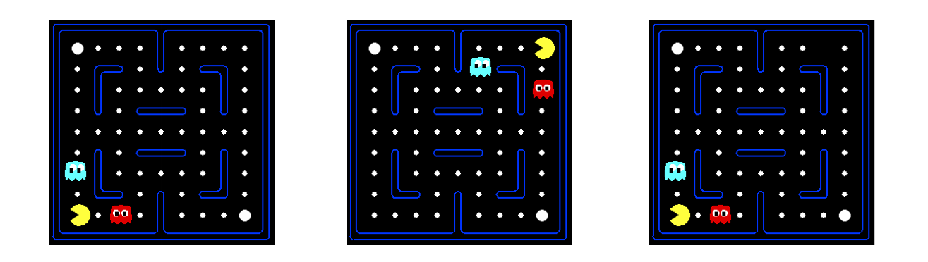
Borrowed from Berkeley's CS188 course, with permission.

Will experiences in any one of the above states inform the agent about the q-values in any of the others?

No! Since, the q-values are stored in tabular fashion, with disparate cells, our agent does not recognize the similarity of these states.

In class, we'll look at some examples of why basic Q-learning is brittle here.

So, we have a problem here: our agent's explored experiences are not being particularly useful for generalizing across similar states with only minor differences.

This is perhaps the single greatest challenge facing AI in the modern era, and is found under the title of transportability.

Transportability is the study of whether or not a policy's behavior in one state is appropriate in a separate one, in which certain aspects may be the same, and others may be different.

So, let's solve AI in the span of the next 5 minutes, shall we?

[Brainstorm] Think of some ways of ensuring greater transportability with the experiences of q-learning agents -- how could we get an agent that was surrounded by ghosts in one part of the board know that this was bad in another part of the board?

We're going to consider a good tradeoff between simplicity and power to address the problem of transportability.

Feature-Based Representations

In the past, we've seen features relevant to some tasks in AI -- what are they and how were they used in the past?

Features are higher-level state characteristics that are constructed from more primitive representations of the state.

How do you think features can help us with the transportability problem?

They can encode *parts* of *different* states that should be treated the same, and then distinguish them when it matters!

With feature-based representations, we can create features that describe the important properties of the state so as to more closely guide our agent on what to pay attention to.

A feature extractor, $f_i(s)$, for some state $s$ and some feature $i$, maps state $s$ to some numeric quantification of desired parts of the state.

What are some example features we may want to extract based on the raw / primitive Pacman board state?

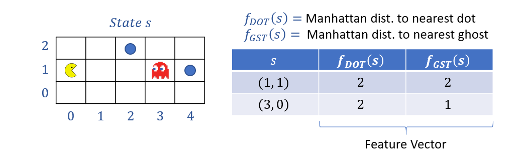
To give but a few...

Distance (in grid cells) from $s$ to the nearest pellet.
Distance (in grid cells) from $s$ to the nearest ghost.
Whether or not Pacman is in a corridor or open space ($0,1$).

Notably, some features are things that we would like to be treated as "good / desirable", others to be treated as "bad."

Moreover, some features may be binary, discrete, or continuous, and we should still be able to assess what they mean for the quality of a particular state.

How, then, would having these features contribute to use knowing the quality of some state?

We can use them to estimate the value function!

Linear Value Functions estimates state values through some linear combination of weighted features. $$V(s) = w_0*f_0(s) + w_1*f_1(s) + ... + w_i*f_i(s)$$

This allows us to not only assess the status of features in any given state, but to then weight them by importance and whether or not they should be treated as good (positive weights) or bad (negative weights).

However, one big issue here is that, as we've seen in the past, knowing state values doesn't particularly help us craft policies on the fly.

Can we adapt the idea of linear state-value functions to aid us in using features for policy formation?

Yes! Just associate features with the qualities of *actions* instead of the *states* and repeat the same procedure!

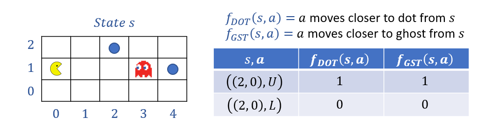
Action feature functions, $f_i(s,a)$, for feature $i$, state $s$, and action $a$, can describe the Q-state and estimate Q-values in the same was as with states.

So, to analogize our features from above, Action Features might look like:

Action $a$ moves closer to a pellet ($0,1$).
Action $a$ moves closer to a ghost ($0,1$).
Action $a$ moves into a corridor ($0,1$).

Likewise, a Linear Action-Value Function estimates action values through some linear combination of weighted action-features. $$Q(s, a) = w_0*f_0(s,a) + w_1*f_1(s,a) + ... + w_i*f_i(s,a)$$

To see why thinking about action-values this way is beneficial:

Pros: we need not track the Q-values of each state-action individually, but instead, summarize the key points with a smaller set of features.
Cons: we may *oversummarize* some states, in which key differences are lost when we switch to the feature-based representation.

Those benefits and risks highlighted, let's think about how to implement these in practice.

Caution: the differences between value-functions and action-value-functions as specified above is a subtle one -- take care that you understand the difference for your final project!

Online, Feature-Based, Approximate Q-Learning

The type of Q-learning we've seen thus-far is what we would call Exact Q-Learning because the values we store in our table will, in expectation, converge to the actual state-action values with enough samples.

To review, those updates during training look like:

We had originally specified the Q-learning update as: \begin{eqnarray} sample &=& R(s, a, s') + \gamma ~ max_{a' \in A(s')}~Q(s', a') \\ Q(s, a) &\leftarrow& Q(s, a) + \alpha~(sample - Q(s, a)) \end{eqnarray}

Merely rewriting some pieces for future convenience, we could re-specify the above as:

\begin{eqnarray} difference &=& sample - Q(s, a) \\ Q(s, a) &\leftarrow& Q(s, a) + \alpha * difference \end{eqnarray}

[Intuition 1] If we were interested in estimating these Q-values instead, we could turn our linear action-value functions into their own learning problem.

What, then, is there to learn through experience with these linear action-value functions?

The weights!

[Intuition 2] By phrasing the q-value estimates in terms of their current belief and the given *differences*, we provide a metric for how wrong our current weights are!

Indeed, we can, through experience, attempt to determine both the magnitude and the positive / negative effect of each feature on the Q-values!

Approximate Q-Learning attempts to learn the weights associated with action-value features through online least-squares (regression).

Thus, the Approximate Q-Learning Weight Update Rule follows from our Exact Q-Learning update, but instead, updates the weights: \begin{eqnarray} difference &=& [R(s, a, s') + \gamma~max_{a'} Q(s', a')] - Q(s, a) \\ w_i &\leftarrow& w_i + \alpha * difference * f_i(s, a) \end{eqnarray}

Note how the difference accounts by how much we were off *and* if we were overestimating (negative) or underestimating (positive). This will then allocate "blame" to each feature based on how large $f_i(s, a)$ was, and whether or not it was negative or positive.

Let's look at some examples!

Examples

Suppose we have an Approximate Q-Learning Agent estimating Q-values with $\alpha = 0.01, \gamma = 1$, and 2 features:

$f_{DOT}(s, a)$, some feature that responds to proximity to a dot.
$f_{GST}(s, a)$, some feature that responds to proximity to a ghost.

Our current weights for these two features (in the present example) are as follows: $$Q(s, a) = 4.0 * f_{DOT}(s, a) - 1.0 * f_{GST}(s, a)$$

Now, suppose we are in some state $s$ (below) in which our current estimate for moving NORTH is $Q(s, NORTH) = 1$, and we haven't yet sampled actions in the state to our NORTH, so for the state $s'$ above $s$, we have $Q(s', a) = 0~\forall~a$.

Since the weight on the dot is quite a bit more than that of the ghost, our agent will more zealously go for the dots than it will avoid the ghosts.

In estimating the Q-value of moving NORTH from $s$, we receive some values for our features, take the action, unfortunately get eaten, and receive a reward of $r = -500$, as depicted below.

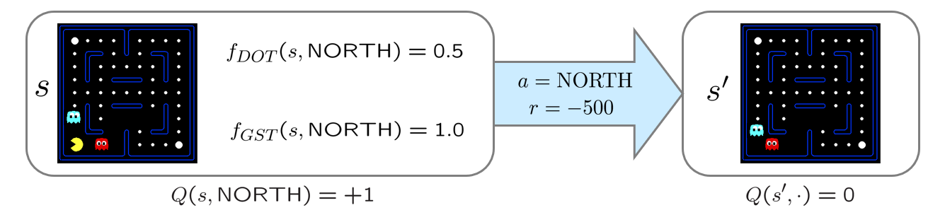
Borrowed from Berkeley's CS188 course, with permission.

The Approximate Q-Learning Update Rule now comes into play since we need to update our weights based on the reward received:

\begin{eqnarray} difference &=& [r + \gamma~max_{a'} Q(s', a')] - Q(s, a) \\ &=& [-500 + 1 * 0] - 1 \\ &=& -501 \\ w_{DOT} &\leftarrow& w_{DOT} + \alpha * difference * f_{DOT}(s, a) \\ &=& 4.0 + 0.01 * (-501) * 0.5 \\ &\approx& 1.5 \\ w_{GST} &\leftarrow& w_{GST} + \alpha * difference * f_{GST}(s, a) \\ &=& -1.0 + 0.01 * (-501) * 1.0 \\ &\approx& -6.0 \end{eqnarray}

Thus, our new linear approximation is: $$Q(s, a) = 1.5 * f_{DOT}(s, a) - 6.0 * f_{GST}$$

So what got accomplished here?

We *reduced* the weight on the dot feature, cautioning our agent to be less reckless in eating.
We *increased* the negative weight on the ghost feature, making our agent realize how bad it is to get caught by them.

Moreover, we were able to do this with a single sample from a single corner of the Pacman maze, which would actually generalize to other areas of the board as well!

In class, we'll take a look at this in action next.

Multi-Agent States

What is perhaps an understated component of the above example is the state $s'$ in which Pacman decided to move Up from $s$, and was then eaten by a ghost.

Note: this $s'$ is thus composed of the environment moving multiple pieces: Pacman moving Up, and *also* the blue ghost moving down!

This distinction is important, especially in turn-based games or when an opponent can act against you, just like the formalization of minimax!

As such, there's a bit of a common mistake in approximate q-learning implementations of which we should be aware:

In multi-agent scenarios, the reward function should evaluate the next state only after all other agent moves have resolved, and the learning agent is able to act again.

To see why this is important, consider environments (like your final project) wherein a reward associated with the agent's choice *ignoring* the opportunity for opponents to act vs. those *incorporating* your opponent are important:

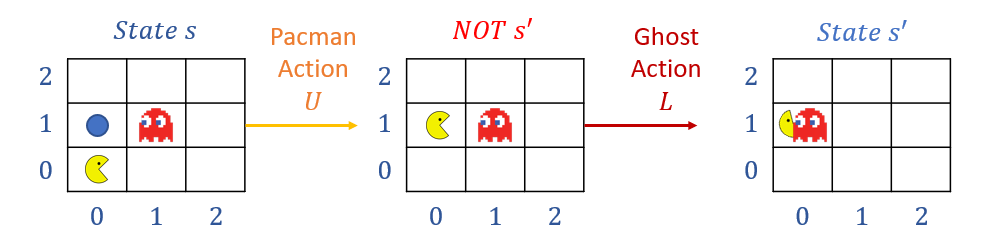
Remarks:

Note how the rewards might be different from the "NOT s'" state (in which Pacman has just eaten a pellet [Good!]) vs. the true State s' (in which Pacman has just been eaten [Bad!]).
In practice, this translates to performing q-value updates *only at the start* of your agent's "turn" to act, keeping a snapshot of the previous s and the now current state s' on which to perform said updates.

So there you have it! Approximate Q-Learning in all its glory.