Practical RL
Let's jot a quick running tab of *every* design decision we might make when fashioning a RL agent:
Reward Function (when not provided by the environment) deciding what values to return based on what state-actions. Moreover, there are a number of sub-decisions to make here, including (but not limited to):
Living rewards
Terminal rewards
Magnitudes (i.e., amounts) and signs (i.e., positive or negative) of each
Discount Factor, deciding how "future thinking" the agent is with rewards
Learning Rate, deciding how quickly to change an agent's valuation, and how to attenuate the learning rate over time.
Policy Formation, model based vs. model free, exact vs. approximate q-learning, exploration vs. exploitation.
So many decisions, so little time -- now you know how your agent must feel!
Today, we'll discuss a few tricks-of-the-trade that help contextualize some of these concerns, while giving you some other, important design decisions that can help create a more intelligent agent.
Reward Shaping
Thus far, we've sort of been assuming the presence of a reward function as though it was magically gifted to us by the environment, and while sometimes it is like with the MAB ad-agents, others, it's up to us as the programmers to describe just when to give a cookie, and when to give a slap on the wrist.
Reward Shaping is the process of crafting a reward function to enable a reinforcement learner to reach desired outcomes with as little training as possible.
The bad news: it's more of an art, than a science, and different problems / objectives demand highly environment-specific tinkering to shape a reward function when the onus of responsibility is in the programmer's hands.
As such we'll look at a few tricks in the sections that follow that provide heuristic direction for how to craft effective rewards.
Sparse vs. Dense Rewards
Consider a real life example that we RL-ify: Suppose there was only 1 reward for your entire college career: +1000 (really? that's it?) for receiving your degree. Why might this be a problem?
You'd probably be doing a *lot* of messing up not knowing what you were doing right / wrong up until the end of 4 years when it really mattered!
What rewards are given instead to address this issue?
Smaller, intermediary ones to give an indication that you're headed in the right direction! +4 for an A (literally, GPA is a reward function lul), +100/100 for a perfect assignment, etc.
This is an important distinction for our agents as well:
Sparse rewards are those given for only a small handful of states / events, whereas dense rewards are given to evaluate the agent in many different states.
Dense rewards are generally preferred, but can often be hard to define; here's how dense rewards are nicer in an extreme example:

I know what you're thinking: "Wait... isn't that cheating?" Yeah kinda!
Here's the thing though: this is why you're in class right now. You *could* spend a long time learning all of the lessons yourself through careful textbook study and massive amounts of discipline... or you could be guided by someone who knows how to show you the path!
These are the differences between sparse and dense rewards.
Why ever have sparse rewards, then, it seems like dense is always better?
Several reasons, but mostly: (1) dense rewards may not be definable or aren't easily so, and (2) their introduction can sometimes lead to unintended consequences...
The Cobra Effect
The biggest risk in designing a reward function is in not really seeing the bigger picture...
Consider the example of what has come to be known as the Cobra Effect, in which unintended consequences arise from a misspecified reward: in India's old British colonies, the government (in an attempt to rid the areas of an infestation of cobras) offered a monetary incentive for people who brought in dead cobras, assuming they'd train populations of mongeese (mongooses?) or w/e to kill them... the population instead started breeding their own cobras to make stocks that they could cash in!
There are some amusing examples of this listed here:
The punchline is that you don't always get what you want, you get what you pay for, and the trick in avoiding that is in:
Careful planning
Testing on small problems to verify functionality before training
Having tools to visualize your rewards before training
Hint: Use the debug visualization tools (debugDraw method) provided in your final project to get a visual gist for your rewards before
full-on training!
Optimistic Sampling
One of the biggest challenges with online q-learning (and approximate q-learning) deals with adequate exploration, and a simple reward shaping trick can be useful to address it (clickbait intro sentence).
What has been our basic means of managing exploration in Q-Learning when our agent is learning online, and what difficulties does this strategy have?
We've been using \(\epsilon\)-greedy thus far (in the assignments), with a random exploration rate; the problem: exploring states that are far from the initial and not exploring particularly intelligently.
Take, for example, the following gridworld, in which there may be some tempting, early terminal states, but a very attractive, distant, and difficult to discover one.
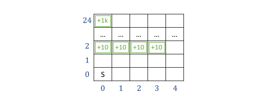
Intuition: There is value in information for exploring not-oft visited states, and a more intelligent explorer should recognize this value.
[Brainstorm] How could we encode this value of information in the exploration / exploitation problem?
There are a variety of different ways to go about this, including some different metrics for value of information.
We'll look at a simple one that produces an optimistic learning agent now.
Exploration Functions
Exploration Functions provide a means of favoring exploration into state-actions that have not been adequately sampled in the past by inflating the q-value of state-actions for which future exploration is desirable.
These exploration functions return an "optimistic utility" for state-actions that allows them to be explored early, but then converges to their true q-value as time goes on.
You'll note an analog to our Thompson Sampling Bandit Player from the MAB section of the course.
A simple exploration-count exploration function is parameterized by a q-value estimate, \(q\), some number of visits to the given state-action, \(n\), and some exploration constant \(K\) (higher means more explanation), we can write the function: $$f(q, n) = q + \frac{K}{n}$$
Using such an exploration function, we provide a new, Optimistic Q-Value Update such that for counter, \(N(s', a')\), which determines how many times we have taken action \(a'\) in state \(s'\), we have an exact Q-Update: \begin{eqnarray} sample &=& R(s, a, s') + \gamma~max_{a'}~f(Q(s', a'), N(s', a')) \\ Q(s, a) &\leftarrow& (1 - \alpha) Q(s, a) + \alpha * sample \\ \end{eqnarray}
Note that the above is for an exact-Q-value update -- in terms of approximate Q-learning, we can still use the exploration function but with the Q-argument for the linear value approximation instead.
In practice, this generally amounts to choosing a value of \(K\) that is larger than the living reward, but smaller than large payouts indicating the states that you most want the agent to attain.
Consider the following gridworld in which the number of times an action has been chosen in state \(s'\) (after taking action \(R\) from \(s\)) are displayed in their respective arrows in \(s'\). Compute the sample value for an exploration constant \(K=2\), \(\gamma = 1\), and \(\alpha = 0.5\).
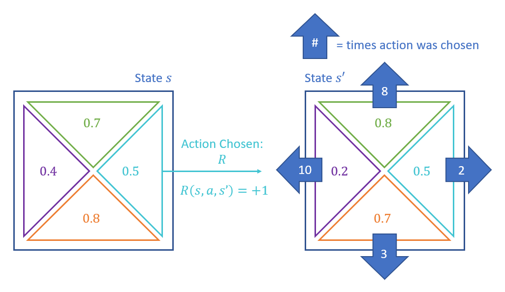
In order to compute the maximizing action \(a'\) for the sample, we have the following exploration function values: \begin{eqnarray} f(Q(s', U), N(s', U)) &=& 0.8 + 2/8 = 1.05 \\ f(Q(s', D), N(s', D)) &=& 0.7 + 2/3 \approx 1.37 \\ f(Q(s', L), N(s', L)) &=& 0.2 + 2/10 = 0.40 \\ f(Q(s', R), N(s', R)) &=& 0.5 + 2/2 = 1.50 \end{eqnarray}
Above, our optimistic sampling result is that \(R\) from \(s'\) maximizes the estimated future reward at this point in the sampling process, so: \begin{eqnarray} sample &=& 1 + 1 (1.5) = 2.5 \\ Q(s,a) &=& 0.5 * 0.5 + 0.5 * 2.5 = 1.5 \end{eqnarray}
Importantly: we would log an additional choice for \(N(s, R)\) after the above sample! In this way, \(f(s, R)\) is reduced upon subsequent choices.
Some things to note about the above:
The only update to the old update rule is how we define the sample, in which the max q-value of the next state is replaced with our optimistic exploration function instead.
Note that as we continue to sample \((s', a')\) over time, the value of \(N(s', a') \rightarrow \infty\), and so the optimistic bonus in the exploration function trends to 0 (i.e., the \(lim_{n \rightarrow \infty}~\frac{K}{n} = 0\)).
This bonus not only influences our perception of the value of the adjacent states to \(s\), but also leads our agent to prefer the states that lead up to the frontier of infrequently explored states (i.e., the bonus propagates to q-values earlier in the action sequence). However, over time, this too attenuates, and the q-values converge to their true values, though with less time to perform the sampling.
Reward Splitting
Disclaimer: This section is still experimental, and is an ongoing exploration in the ACT Lab! We've seen positive experience with it thus far.
Recall from our introductory lecture that we motivated the many primary rewards that humans receive in response to their actions, e.g.

Are the features / actions we associate with each of the above rewards the same?
No! The features / actions we take to sate hunger are different than, e.g., scratching an itch or drinking to sate thirst (there's probably a "thirst" pun here for the sex reward but I'll abstain pre-tenure).
Just as we as humans manage our behaviors in response to many complex rewards and totally separate cognitive processes, so too can it be beneficial to think about separating the rewards to which our agents respond and learn.
Consider the following Pacman example in which Pacman moves onto a tile containing a pellet and eats it (good!) but then before he can act again, is eaten by a ghost (bad!).
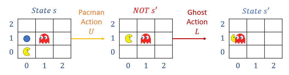
Suppose the reward signal was configured to receive a +100 for eating a pellet and a -500 for dying, for a net of \(R(s, a, s') = -400\). Now, suppose we had two state-action-features related to proximity to ghost / pellet with pre-move weights: $$Q(s, a) = 1.0 * f_{DOT}(s, a) - 1.0 * f_{GST}(s, a)$$ ...and post-sample weights of: $$Q(s, a) = -1.0 * f_{DOT}(s, a) - 2.0 * f_{GST}(s, a)$$ [!] Note: the weight on \(f_{DOT}\) has now switched signs.
What's the problem with the above if \(f_{DOT}\) is a feature that is meant to guide Pacman to eat the pellets?
It now has a negative weight, which will make Pacman pellet-intolerant!
This unintended effect wherein multiple aspects of the reward signal are encountered at once -- at least Pacman had his last meal before getting ghosted!
The above is an instance of a larger problem (that we'll discuss in the 2nd half of the course) known as the Attribution Problem, wherein it can be ambiguous as to what parts of the state were the causal explanation for some witnessed effect.
In the above example, both proximity to a pellet AND proximity to a ghost got the blame for the big -400, and in general, this can't be always avoided (we as humans struggle with this too, e.g., was it that restaurant you ate at that made you vomit, or the tequila binge you had the night prior?).
Taking inspiration from the above, what might we do to ameliorate the attribution problem with feature-based Q-learning?
Split the different reward signals into pieces to which only certain features respond!
Reward Splitting is a type of reward shaping wherein we split a single reward value into multiple heterogeneous rewards, each with their own composite features, weights, and updates.
For instance, splitting our original \(R(s, a, s')\) above into measures of satiety for eating pellets, \(R_{EAT}(s, a, s')\) and getting eaten by ghosts \(R_{DED}(s, a, s')\), we can thus form different Q-estimates based on different features: \begin{eqnarray} Q_{EAT}(s, a) &=& w_{DOT} * f_{DOT}(s, a) \\ Q_{DED}(s, a) &=& w_{GST} * f_{GST}(s, a) \\ \end{eqnarray}
Notes on the above:
In the instance of the transition in the example above (with the -400 reward), we would instead assign a vectorized reward of \(\langle R_{EAT}, R_{DED} \rangle = \langle 100, -500 \rangle \).
Updates to \(w_{DOT}\) would thus be sensitive to the +100 reward, and updates to \(w_{GST}\) by the -500.
Had we more features / rewards, we can continue to add them to these split reward signal q-estimates.
Suppose we do split our reward like the above, what must we still remember to do in order to characterize what the *best* action is in any given state?
Have some means of recombining the individual signals!
A pooling function \(F(Q_{0}(s, a), Q_{1}(s, a), ...) = \hat{Q}(s, a)\) provides a means of combining the split reward signals and associated q-estimates such that we gain an estimate of the holistic Q-value, \(\hat{Q}(s, a)\) on which to maximize: \(\pi^*(s) = argmax_a \hat{Q}(s, a)\).
This can be as simple as a sum of the individual signals, or something more sophisticated like a weighted sum of some sort (not sure how though, this is an open topic of research!).
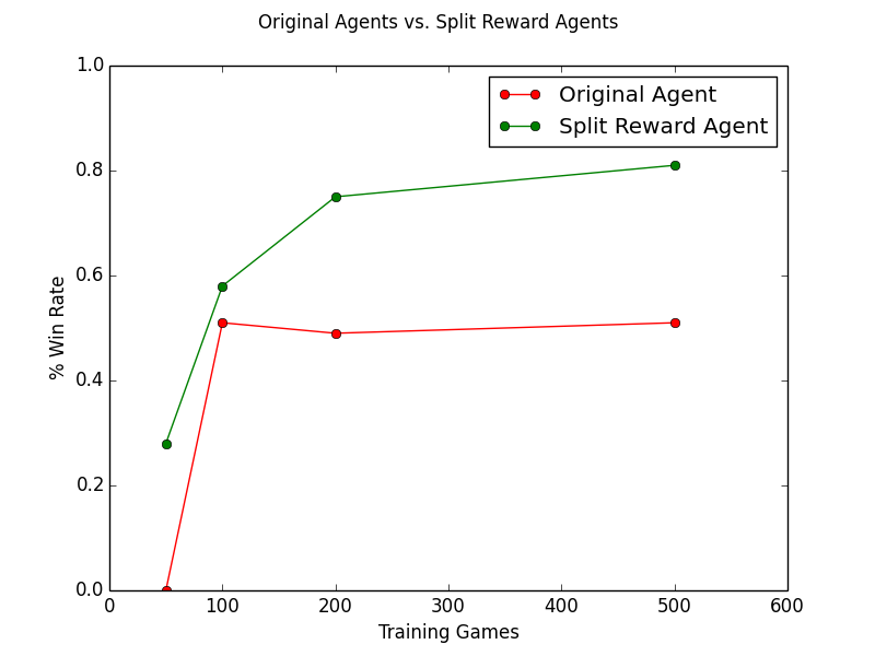
Here are some cool preliminaries from our very own ACT Lab researcher Lucille Njoo, demonstrating the percentage of won games with the same features split across multiple reward signals compared to one on just a single Pacman agent on the final project.
And there you have it! Some split rewards to make things a bit easier on your little learner.
Policy Search
The above addresses issues with adequately sampling the actual q-values for any state-action pair, but we've seen, in the past, where this might not be the most important thing to do for good agent performance.
Just as before, when we performed policy-iteration as an alternative to value-iteration, we can consider doing something similar for the domain of q-learning.
Intuition: feature-based q-learners that provide good estimates for q-values may not necessarily translate into good policies!
This can be for a variety of reasons, though typically:
The feature-based representations may over-summarize important differences between states that might otherwise look identical from the features' perspective.
The reward function may be poorly specified.
If we care *mostly* about the agent's performance, we can instead focus on tweaking the weights associated with features based on an objective function related to their cumulative reward.
This iterative improvement is a form of hill-climbing known as policy-search with an objective function of cumulative reward.
The steps of Policy Search are as follows:
Learn feature weights by approximate q-learning to produce a baseline policy \(\pi_0\).
Tweak features weights by tenets of hill climbing (increment / decrement by some step size) to produce some \(\pi_{i}\) (for iteration \(i \gt 0\)).
Evaluate policy \(\pi_i\) (see its cumulative reward over many episodes, like through TDL).
Repeat until some stopping condition met.
While policy search is useful and produces typically better policies than naive q-learning / approximate q-learning alone, it also has some weaknesses.
What are some weaknesses of policy search?
Chiefly: The policy evaluation step can take a long time, and with many features in the feature vector, can be impractical for hill-climbing to fix.
Andrew's Forecast: This might be a good venue for exploring the applicability of causal inference! CI can help decompose the states and define some sort of counterfactual gradient to help improve it.