Last lecture we started to see some of the shortcomings in Bayesian Networks (BNs) to answer more nuanced queries of a causal nature.

Instead, we need some stronger causal assumptions about the system in order to answer these interesting queries.

As such, today we take our first steps towards the next wrung in the causal hierarchy -- look at that little fellow climb!

So, as we ascend the causal ladder, let's start by thinking about the new tools we have, the properties of the tools we need, and how we can start to address the issues raised with Bayesian Networks for Causal Queries that we discussed last class.

Zooming out real quick, we should give some context for what we're trying to do and what the pieces are:

A causal inference engine is a combination of several components that can (potentially) be used to answer queries at PCH tiers above the associational: chiefly, (1) a causal model of the environment, (2) some data, and (3) some query of interest, or pictorially:

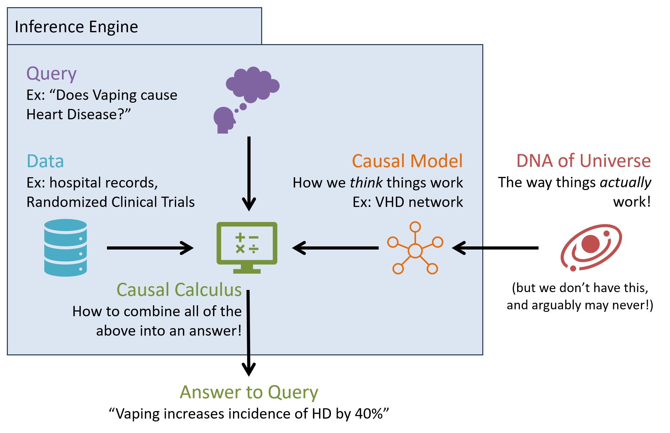
Importantly, a reminder: many causal queries cannot be answered from data alone! We require a causal model to state our assumptions about how the world works, through which we can then interpret data to answer a query.

So, with this perspective established, we know that we can't use a basic Bayesian Network for our causal model, but there's a good amount there that maybe we can draw inspiration from.

Whatever approach / model we use to answer causal questions should have an answer to issues we saw with using Bayesian Networks for Causal queries we established from the last lecture:

• Observational equivalence of associative models can induce different causal structures can have the same statistical dependencies.

• Confounding bias of associational tools like conditioning contaminate the answers to causal queries.

• Unobserved confounders can represent parts of the model we're missing that might create this confounding bias.

In this lecture, we'll consider remedies to the first two points, and leave the subtler points of the third for future discussion.

Let's start with the most fundamental guideline of causality

A Structural Causal Model (SCM) specifies the modeler's assumptions about a system of cause-effect relationships, and is formalized as a 4-tuple \(M = \langle V, U, F, P(u) \rangle \) consisting of the following components:

I. \(U\), Exogenous Variables: a set of variables \(U = \{U_0, U_1, ..., U_u\}\) whose causes are outside of the model.

Exogenous variables are also the sources / inputs of noise or other inputs outside of the model.

You can remember these as variables whose states are decided by factors outside of, i.e., external to, the SCM, even though these factors likely exist in the true model of reality, which we are merely sampling.

II. \(V\), Endogenous Variables: a set of variables \(V = \{V_0, V_1, ..., V_i\}\) whose causes are known -- either as exogenous or other endogenous variables.

Endogenous variables are those that we are claiming to have the "full picture" on, though any variance in their state can be attributed through exogenous parents or ancestors.

III. \(F\), Structural Equations: a set of functions \(F = \{f_{V_0}, f_{V_1}, ..., f_{V_i}\}\) for each endogenous variable that describes how each variable responds to its causes.

The vocabulary of "cause" is thus dictated by these structural equations: if a variable \(X\) appears as a parameter to another's \((Y)\) structural equation, then we say that \(X\) is a direct cause of \(Y\): $$Effect \leftarrow f_{Effect}(Causes)$$

Note: these functions can describe any relationship and are not limited to probabilistic expressions.

They are called "structural" because they are meant to uncover / model the "structure" of causes and effects in the system, and exhibit some nice, causal properties that we'll see in a moment.

Note the arrow "assignment" operator above that demonstrates an important assymetry: the child / effect *gets* its value from its parents, but we cannot use this like an equation, moving terms freely from one side of the operator to the other.

Consider our VHD network in a more simplified, rule-based SCM like the following:

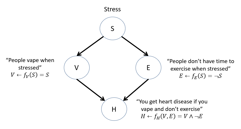
Why no structural equation for Stress?

Because it's an exogenous variable -- its causes are decided by factors we didn't / couldn't include in the model!

So how to determine its value if not through a structural equation?

Since exogenous variables represent the entry-point for noise / probability in the system, just model its state as a distribution, \(P(u)\)

IV. \(P(u)\), Probability Distributions Over All \(u \in U\): because exogenous variables' causes are unobserved, we can only speculate about their state through some probability distribution assigned to each. Additionally, since all endogenous variables have at least 1 exogenous ancestor, \(P(u)\) elicits a probability distribution over \(P(v|parents(v))~\forall~v \in V\).

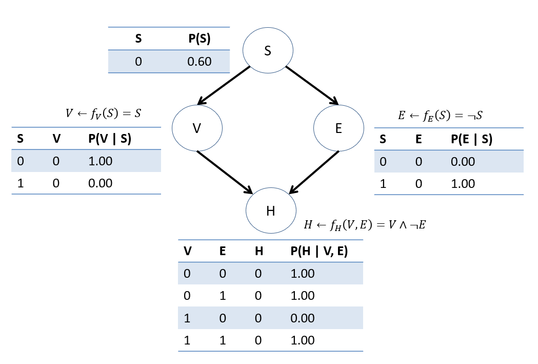
Consider how we could convert each of the structural equations from the previous VHD SCM into CPTs on each node.

By defining \(U\) and \(P(u)\) as distinguished from \(V\), we cleanly separate the sources of noise in our model from the sources of causal information.

Important notes for the above:

• Some endogenous variables may have both exogenous and endogenous parents, others may only have endogenous.

• If we *did* know the state of every exogenous variable, we could determine the state of any \(V\) in the model with perfect accuracy (in theory, at least!), even though we must represent the exogenous causes probabilistically.

Between specifying \(F, P(u)\), and deriving \(P(v|parents(v))~\forall~v \in V\), we can then perform associational inference in the same way as a Bayesian network using tools like enumeration inference!

In the present example, this is fairly trivial because of the CPT probabilities, but as an exercise, you can try deploying full enumeration inference on the following:

Find \(P(H=1)\).

Just analytically, we can see that this happens any time \(P(S=1)\), which would thus be \(0.4\) from the \(P(u) = P(S)\) distribution.

Find \(P(H=1|V=1)\).

Interestingly now, if \(V = 1 \Rightarrow S = 1 \Rightarrow E = 0\), and so \(P(H=1|V=1) = 1\)... with certainty!

BUT... does this mean we should put the vapes down? Well... maybe...

Remember this is just an associational query, so what we've effectively said in this totally-not-an-ad-for-the-Truth-campaign is that 100% *of those who vape* will get heart disease... not necessarily that vaping is its cause!

We'll need some stronger tools to answer that.

Causal Endeavors

---

Causal models appear in two main fields at the intersection of AI, Machine Learning, Statistics, and the Empirical Sciences (even some philosophy as well!):

In Causal Induction / Discovery, the objective is to learn the causal graph, generally from some offline dataset, but increasingly from the experience of learning agents as well.

Depicted, causal discovery is concerned with taking some data and being able to assert the cause-effect relationships from it:

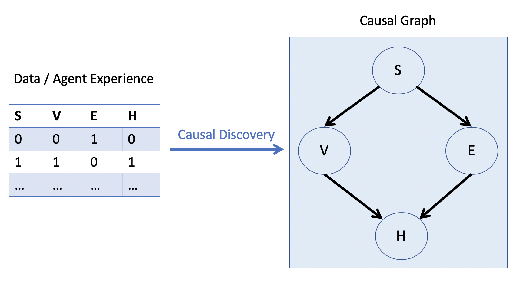
The Type of data matters heavily for causal discovery (e.g., if we have associational vs. interventional data), which we'll discuss next class.

Causal discovery is a very difficult problem when analyzing offline, observational data, and generally requires much domain knowledge, compromise, and strong assumptions to automate.

The upshot: intelligent agents who can interact with their environments have an easier time of it, which is why this course compares causality with reinforcement learning!

Apparently the people at Deep Mind agree; here's a recent article on the matter (small flex: they even cite me):

Causal Reasoning from Meta-reinforcement Learning

Personally, I believe this union is a great avenue for further research, so as this course progresses, feel free to share your thoughts, questions, and suggested explorations!

Now, either discovered or assumed, what do we do with causal models?

In Causal Inference, it is assumed that the Causal Model is known / correct, and then is employed in answering causal and (if capable) counterfactual queries of interest.

Causal inference will be the main topic of this course, but there's plenty to be said on both -- we'll see some examples of each as we continue in the course.

Let's start by flexing our first new tool from the causal arsenal: tier-2 up up and away!

Returning to our Vaping-Heart Disease (VHD) example, for now, let's suppose we're happy with our original SCM and are able to (for now, hand-wavingly) defend it as a correct model of the environment. Let's attempt to answer the causal question: "Does vaping cause heart disease?"

Supposing our SCM is correct, we still have a problem with the Bayesian conditioning operation for examining the difference in conditional probabilities.

To remind us of this problem:

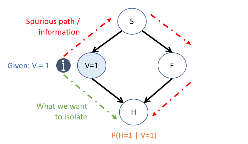
[Reflect] How can we isolate the effect of \(V \rightarrow H\) using just the probabilistic parameters in our CBN?

I dunno... how about we just chuck the "backdoor" path?

More or less, yeah! That's what we're going to do through what's called an...

Intervention

---

I know what you're thinking... and for any Always Sunny fans out there, I have to reference with:

In our context, however...

Intuition 1: Causal queries can be thought of as "What if?" questions, wherein we measure the "downstream" effect of forcing some variable to attain some value apart from the normal / natural causes that would otherwise decide it.

An intervention is defined as the act of forcing a variable to attain some value, as though through external force; it represents a hypothetical and modular surgery to the system of causes-and-effects.

As such, here's another way of thinking about causal queries:

With this intuition, we can rephrase our question of "Does vaping cause heart disease" as "What if we forced someone to vape? Would that change our belief about their likelihood of having heart disease?"

Because observing evidence is different from intervening on some variable, we use the notation \(do(X = x)\) to indicate that a variable \(X\) has been forced to some value \(X = x\) apart from its normal causes.

The effect of interventions in an SCM for, say, \(do(X=x)\) is to replace the structural equation of \(X\) with the fixed value, viz.: $$do(X=x) \Rightarrow X \leftarrow f_X(...) = x$$ The effects of this replacement then appear in every descendant structural equation.

Heh... do.

Obviously, forcing someone to vape is unethical, but it guides how we will approach causal queries, as motivated by the second piece of intuition:

Intuition 2: Because we're asking causal queries in a CBN, wherein edges encode cause-effect relationships, the idea of "forcing" a variable to attain some value modularly effects only the variable being forced, and any descendant variables, and should not affect any other cause-effect relationships.

This will be an important question later, since intelligent agents may need to predict the outcomes of their actions regarding how they change *parts* of the state, but not others.

If an intervention forces a variable to attain some value *apart from its normal causal influences,* what effect would an intervention have on the network's structure?

Since any normal / natural causal influences have no effect on an intervened variable, and we do not wish for information to flow from the intervened variable to any of its causes, we can sever any inbound edges to the intervened-upon variable!

Let's formalize these intuitions... or dare I say... in-do-itions (that'll be funny in a second).

Structurally, the effect of an intervention \(do(X = x)\) creates a "mutilated" subgraph denoted \(G_{X=x}\) (abbreviated \(G_x\)), which consists of the structure in the original network \(G\) with all inbound edges to \(X\) removed.

So, returning to our motivating example, an intervention on the Vaping variable would look like the following, structurally:

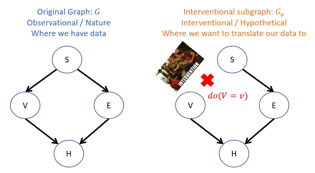
Some notes on the above:

• The original graph represents how things operate normally in reality whereas the interventional subgraph is in the world of "what if".

• That said, sometimes we can actually measure the interventional side of things by conducting a randomized experiment (more on that later).

This is how we proceduralize a "What if?" question!

To add to that vocabulary, for artificial agents, an observed decision is sometimes called an "action" and a hypothesized intervention an "act".

"HEY! That's the name of your lab! The ACT Lab!" you might remark... and now you're in on the joke.

Interventional Inference

---

So returning to our example, we are hypothesizing the effect of vaping on other variables in the system.

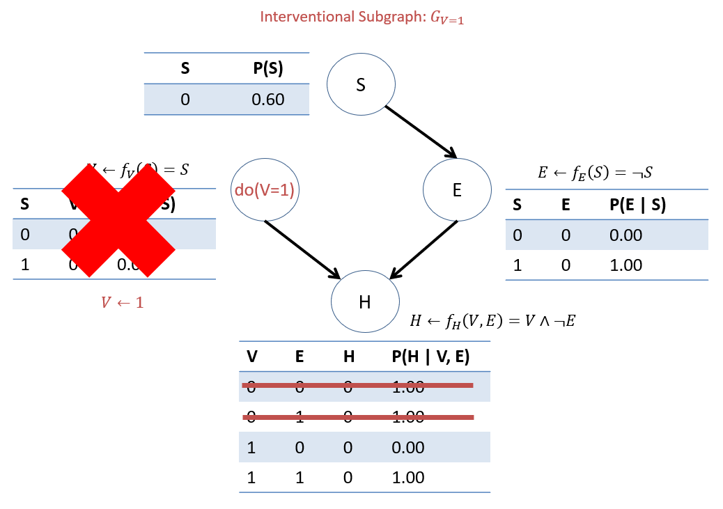
The only asymmetry we thus introduce is that by forcing \(do(V = v)\), we replace the CPT for \(V\) and instead have \(P_{G_{V}}(V = v) = 1\), and then have \(V=v\) in all other CPTs mentioning \(V\).

Consider the Markovian Factorization of the original network (repeated below); how would this be effected by an intervention \(do(V = v)\)? $$P(S, V, E, H) = P(S)P(V|S)P(E|S)P(H|V,E) = \text{MF in Original Graph}$$ $$P(S, E, H | do(V = v)) = P_{G_{V=v}}(S, E, H) = \text{???} = \text{MF in Interventional Subgraph}$$

Since we are forcing \(do(V = v)\) (i.e., \(V = v\) with certainty apart from its usual causes), this is equivalent to removing the CPT for \(V\) since \(P(V = v | do(V = v)) = 1\). As such, we have: $$P(S, E, H | do(V = v)) = P_{G_{V=v}}(S, E, H) = P(S)P(E|S)P(H|V=v,E)$$

Observe the effect of intervening on \(do(V=1)\) in our VHD SCM:

This motivating example is but a special case of the more general rule for the semantic effect of interventions:

In a Markovian SCM (defined as SCMs where there are no unobserved confounders), the Truncated Product Formula / Manipulation Rule is the Markovian Factorization with all CPTs except the intervened-upon variable's, or formally: $$P(V_0, V_1, ... | do(X = x)) = P_{X=x}(V_0, V_1, ...) = \Pi_{V_i \in V \setminus X} P(V_i | PA(V_i))$$

Example

---

You knew this was coming, but dreaded another computation from the review -- I empathize, this is why we have computers.

That said, it's nice to see the mechanics of causal inference in action, so let's do so now.

Using the heart-disease BN as a CBN, compute the likelihood of acquiring heart disease *if* an individual started vaping, i.e.: $$P(H = 1 | do(V = 1))$$

As it turns out, the steps for enumeration inference are the same, with the only differences being in the Markovian Factorization now being the Manipulation Rule; in other words: just do enumeration inference in the world where some intervened variable \(do(D=d)\) is forced to some value! $$P(Q | do(D=d), E=e) = P_{G_d}(Q | e)$$

And there you have it! Our first steps into Tier 2 of the Causal Hierarchy.

But wait! We didn't *really* answer our original query: "What is the *causal effect* of vaping on heart disease?"

To answer the question of what effect Vaping has on Heart Disease, we can consider a mock experiment wherein we forced 1/2 the population to smoke and the other 1/2 to abstain from smoking, and then examined the difference in heart disease incidence between these two groups!

Sounds ethical to me! </s> </dangling-tags>

We'll talk more about sources of data and the plausible estimation of certain queries of interest in the next class.

That said, this causal query has a particular format...

Average Causal Effects

---

The Average Causal Effect of some binary intervention \(do(X = x)\) on some set of query variables \(Y\) is the difference in interventional queries: $$ACE = P(Y|do(X = 1)) - P(Y|do(X = 0))$$

So, to compute the ACE of Vaping on Heart disease (assuming that the CBN we had modeled above is correct), we can compute the likelihood of attaining heart disease from forcing the population to Vape, vs. their likelihood if we force them to abstain: $$P(H=1|do(V=1)) - P(H=1|do(V=0)) = 0.4 - 0.0 = 0.4$$

Wow! Turns out the ACE of vaping is a \(+40\%\) increase in the chance of attaining heart disease!

Risk Difference

---

It turns out our original, mistaken attempt to measure the ACE using the Bayesian conditioning operation was not causal, but still pertains to a metric of interest in epidemiology:

The Risk Difference (RD) is used to compute the risk of those already known / observed to meet some evidenced criteria \(X = x\) on some set of query variables \(Y\), and is the difference of associational queries: $$RD = P(Y|X = 1) - P(Y|X = 0)$$

Computing the RD of those who are known to Vape on Heart Disease, we can compute the risks associated with those who Vape vs. those who do not: $$P(H=1|V=1) - P(H=1|V=0) = 1.0 - 0.0 = 1.0$$

Intuiting the above:

• From the ACE: The *actual* causal effect of vaping increases the average person's risk of heart disease by \(40\%\)

• From the RD: Amongst those who were already observed vaping / were not forced to vape but do, together with their vaping habit, the system of other causes and effects suggest that they will certainly get heart disease.

All of today's (lengthy!) lesson seems to hinge on our models being correct, and as we'll see, on the data supporting them. Next time, we'll think about how we might still be able to answer queries of interest even if there are some quirks in either. Stay tuned!

Conceptual Miscellany

---

How about a few brain ticklers to test our theoretical understanding of interventions?

Q1: Using the heart disease example above, and without performing any inference, would the following equivalence hold? Why or why not? $$P(H = 1 | do(V = 1), S = 1) \stackrel{?}{=} P(H = 1 | V = 1, S = 1)$$

Yes! This is because, by conditioning on \(S = 1\), we would block the spurious path highlighted above by the rules of d-separation. As such, these expressions would be equivalent. This relationship is significant and will be explored more a bit later.

Q2: would it make sense to have a \(do\)-expression as a query? i.e., on the left hand side of the conditioning bar of a probabilistic expression?

No! The do-operator encodes our "What if" and is treated as a special kind of evidence wherein we force the intervened variable to some value; as this is assumed to be done with certainty, there would be no ambiguity for it as a query, and therefore this would be vacuous to write.

Q3: could we hypothesize multiple interventions on some model? What would that look like if so?

Sure! Simply remove all inbound edges to each of the intervened variables, and then apply the truncated product rule to remove each of the intervened variables' CPTs from the product!

Each of the above will fuel some future tools we'll need for the deeper dive into causality... those and more, next time!