Causal Bayesian Networks
Last class we saw our, admittedly rigid, Structural Causal Model (SCM) for the Vaping-Heart-Disease scenario, as depicted below:
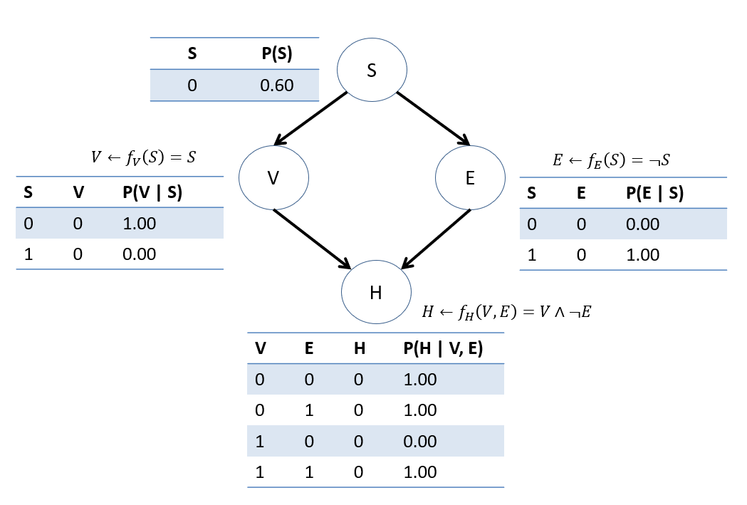
What part(s) of this model are not particularly realistic / feasible to know in practice?
Knowing the *true* \(F\) for the system in reality! Moreover, the ones we chose above are pretty darn simplistic; if you're stressed, then you vape? There are a lot of other variables that probably factor into our decisions!
Add some more exogenous variables that might explain the endogenous factors in the VHD SCM above.
Some examples might include:
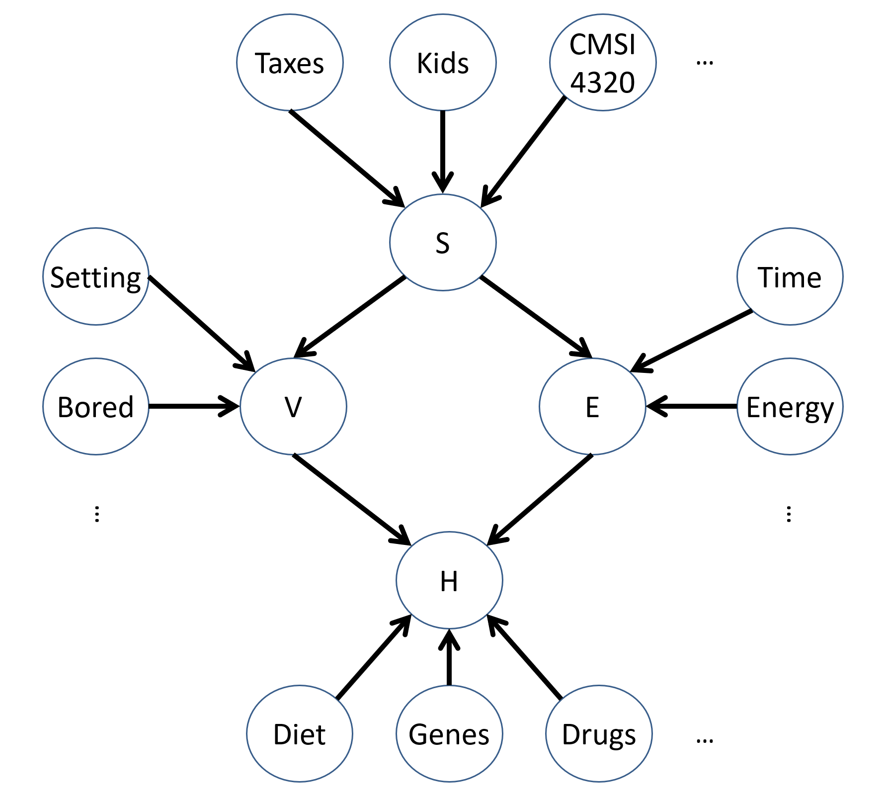
What would the NEW structural equations, \(F\), look like in the modified model above?
Who knows! That's getting really complex, and assumes we haven't missed anything with the variables we added above.
Still: us humans will give explanations in a similar fashion to the above! E.g., try to answer the question "What factors decide whether or not you go to the gym on a given day?"
(equally valid answers include: "will not attend if current day ends in '-day'")Yet, we shouldn't also disparage models where we do know all of the pieces, these can also crop up!
Can you think of some scenarios wherein we *may* know the true structural equations?
Modeling logical problems, rules in simulations / video games (wherein the programmers are "god"), known laws of physics / chemistry, econometrics where rates of exchange / prices are set or known, etc.
This does not mean that lacking structural equations sinks us; there is still merit in knowing which variables we would like to model as causes of which other variables, even if we do not know precisely *how* they affect one another.
By way of some definitions from the above, there are two distinctions of SCMs from how we define / know the structural equations \(F\):
Fully-Specified SCMs: the full structural equations, including which are parameters to which others, are known.
Partially-Specified SCMs: the model indicates which variables are parameters to which other's structural equations, but does not know what those equations are, precisely
In a nutshell: having the exact structural equations is nice and allows for powerful prediction, but when we lack them, it may not be the end of the world...
How could we still use a partially-specified SCM for causal inference?
You've pretty much got two options: (1) try to learn the functions somehow or (2) in their absence, simply express the causal relationship probabilistically -- just use CPTs to encode all of the missing variables, even the ones you don't know!
Consider the following simple example of reasons why you might exercise (E) when we know or don't know all of the reasons (in this example: 2 reasons being Stress (S) and having free time (T)).
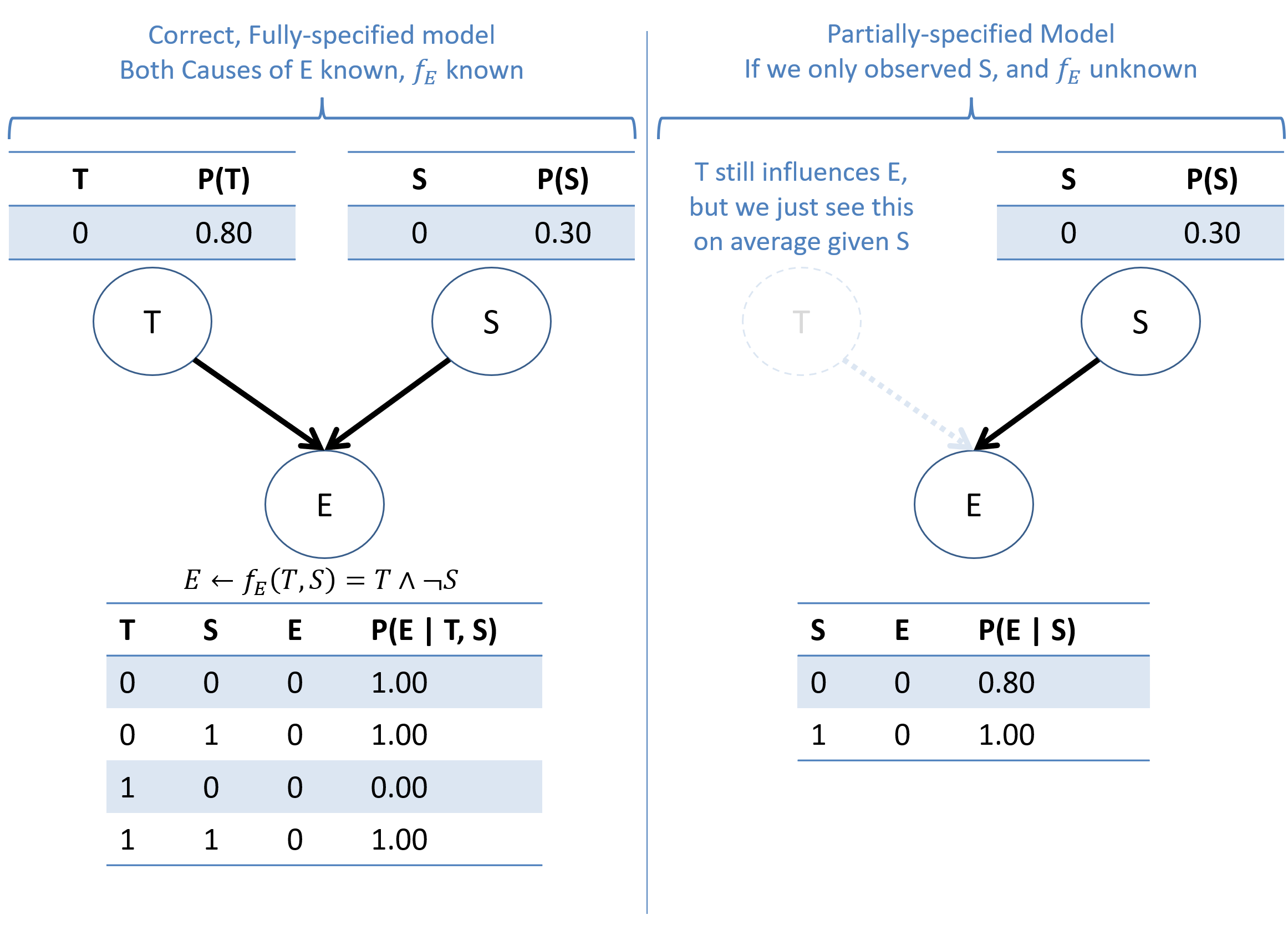
Computing the above using our rules of probability calculus:
\begin{eqnarray} P(E=0 | S=0) &=& \sum_t P(E=0 | S=0, T=t) P(T=t) \\ &=& P(E=0 | S=0, T=0) P(T=0) + P(E=0 | S=0, T=1) P(T=1) \\ &=& 1.0 * 0.8 + 0.0 * 0.2 \\ &=& 0.8 \\ P(E=0 | S=1) &=& \text{(...left as an exercise...)} \\ &=& 1.0 \end{eqnarray}
As such, we now see a type of SCM that has some slightly lesser informational power, but can still give us the ability to answer tier-2 queries!
A Causal Bayesian Network (CBN) is a type of Partially-specified Structural Causal Model (SCM) that behaves precisely like a Bayesian Network but with the guarantee that its structure encodes correct causal relationships.
Necessary conditions for a Bayesian Network to be considered Causal:
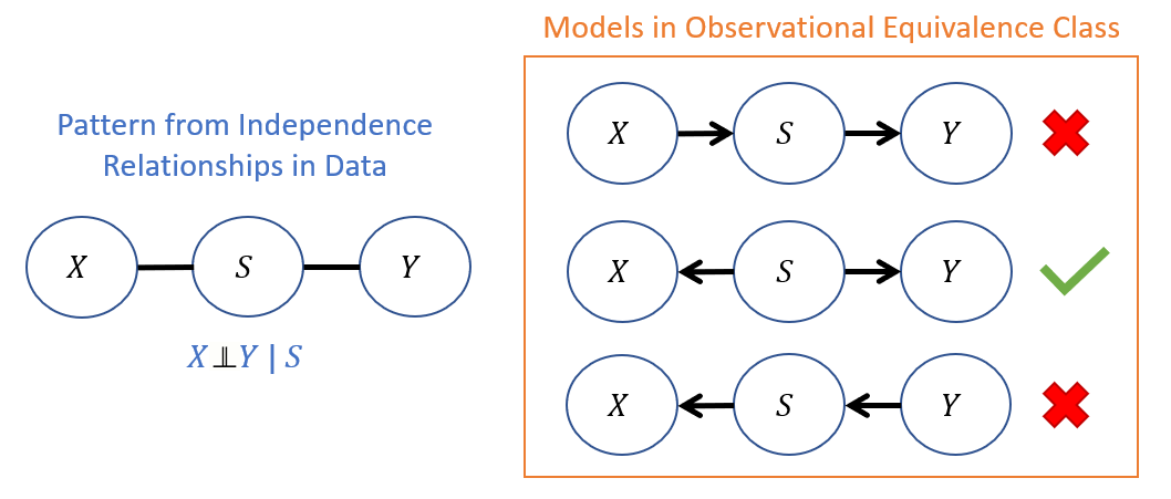
It exhibits the Global Markov Property, meaning that the CBN structure \(G\) encodes independence relationships that are faithful to the underlying data, namely: $$X \indep Y~|~Z~\Leftrightarrow~G.dsep(X, Y, Z)$$
The CBN structure \(G\) is either the *only* structure in the observational equivalence class that encode the independence relations in the data, or is the only one that is not excluded on other scientific grounds.
Consider the following example in which an individual's sex assigned at birth, \(S\), covaries with two other variables \(X = \text{height}, Y = \text{weight}\) but for which \(X \indep Y~|~S\). This elicits the following set of models in its observational equivalence class, only one of which can carry causal meaning because sex cannot be affected by one's height or weight.
Reminder / Tagline: Causal Queries require Causal Assumptions that we encode in the causal model's structure!
CBN Interventions
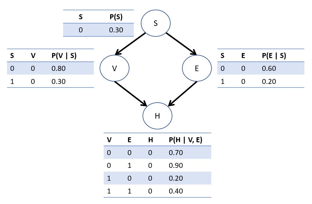
Consider now that the original BN we had on the VHD network was indeed causal (i.e., satisfies the properties of a CBN above)! Let's remind ourselves of its CPTs.
We can repeat our intervention steps from the fully-specified SCM example now in the context of a CBN, but let's see how things work with both *observations* AND *interventions*.
Using the heart-disease BN as a CBN, compute the likelihood of acquiring heart disease *if* an *already stressed* individual started vaping, i.e.: $$P(H = 1 | do(V = 1), S = 1)$$
As it turns out, the steps for enumeration inference are the same, with the only differences being in the Markovian Factorization now being the Manipulation Rule; in other words: just do enumeration inference in the world where some intervened variable \(do(D=d)\) is forced to some value! $$P(Q | do(D=d), E=e) = P_{G_d}(Q | e)$$
Step 1: Labeling variables, the only difference being that we track the tier-1 observed variables \(e\) separately from the tier-2 intervened variables \(d\): $$Q = \{H\}, e = \{S = 1\}, d=\{do(V = 1)\}, Y = \{E\}$$
Thus, we see that our target query lacks any observed evidence at all, and is simply: $$P(H = 1 | do(V = 1), S = 1) = P_{G_{V=1}}(H = 1 | S = 1)$$
Step 2: \(P_{G_d}(Q, e)~\forall~q \in Q\) Now that we have some observed evidence, unlike our previous example in the fully-specified SCM, we'll need to compute this query for all values of \(q \in Q\), giving us the need to find: \(P_{G_{V=1}}(H = h, S = 1)\) \begin{eqnarray} P_{G_{V=1}}(H = 0, S = 1) &=& \sum_{e} P_{G_{V=1}}(H = 0, S = 1, E = e) \\ &=& P(S = 1) \sum_{e} P(E = e | S = 1) P(H = 0 | V = 1, E = e) \\ &=& P(S = 1) [P(E = 0 | S = 1) P(H = 0 | V = 1, E = 0) \\ &+& P(E = 1 | S = 0) P(H = 0 | V = 1, E = 1)] \\ &=& 0.4 * [0.2 * 0.2 + 0.4 * 0.4] \\ &=& 0.08 \\ P_{G_{V=1}}(H = 1, S = 1) &=& P(S = 1) [P(E = 0 | S = 1) P(H = 1 | V = 1, E = 0) \\ &+& P(E = 1 | S = 0) P(H = 1 | V = 1, E = 1)] \\ &=& 0.4 * [0.2 * 0.8 + 0.4 * 0.6] \\ &=& 0.16 \\ \end{eqnarray}
Step 3: \(P_{G_v}(e) = \sum_q P_{G_v}(Q=q, e)\) Thus why we compute step 2 for all values of the query -- makes this one easy! \begin{eqnarray} P_{G_{V=1}}(S = 1) &=& \sum_h P_{G_{V=1}}(H = h, S = 1) &=& 0.08 + 0.16 &=& 0.24 \end{eqnarray}
Step 4: \(P(Q|do(v), e) = P_{G_v}(Q | e) = \frac{P_{G_v}(Q, e)}{P_{G_v}(e)}\) Normalize!
\begin{eqnarray} P_{G_{V=1}}(H = 1 | S = 1) &=& \frac{P_{G_{V=1}}(H = h, S = 1)}{P_{G_{V=1}}(S = 1)} &=& \frac{0.16}{0.24} &=& \frac{2}{3} \end{eqnarray}
Comparing Tier-1 + 2 Queries
Left as an exercise, but if you computed JUST \(P(H = 1 | do(V = 1))\) on the example CBN above, you'd find the answer to be \(0.664\), which is still DIFFERENT from observational \(P(H = 1 | V = 1) = 0.650\).
Let's compare the associational and interventional quantities we had from our original BN with these same CPTs earlier:
Associational / Observational: "What are the chances of getting heart disease if we observe someone vaping?" $$P(H = 1 | V = 1) = 0.650$$
Causal / Interventional: "What are the chances of getting heart disease *were someone* to vape?" $$P(H = 1 | do(V = 1)) = 0.664$$
Hmm, well, doesn't seem like a huge difference, does it -- a mere ~1.5% is all we have to show for our pains?
Although it may not seem like a lot, keep the following in mind:
This is a small network, and therefore, little chance for things to go completely haywire. In larger systems with different parameterizations, these query outcomes can be much more dramatically different.
Note also the difference in information passed through spurious paths in the network based on the associational vs. causal queries (depicted below).
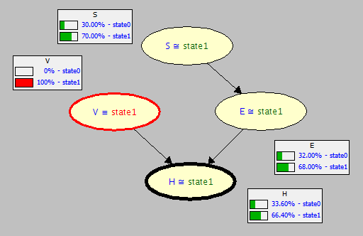
Note the CPTs for each node updated for observing \(V = 1\) in the original graph \(G\).

Now, note the CPTs for each node updated (or lack thereof) for intervening on \(do(V = 1)\) in the mutilated subgraph \(G_{V=1}\).