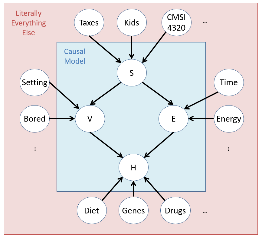
Latent / Unobserved Variables
Last lecture, we started exploring Causal Bayesian Networks (CBNs) as a form of partially-specified SCM that could be used to soften the requirement of knowing the precise structural equations that govern the system's variables.
As it turned out, the reason we use CPTs on all variables in a CBN is due to the influence of other variables that affect ours and are not captured in the causal model, which are known as Latent Variables.
Latent / Omitted / Unobserved Variables are those that affect the observed variables of the system but whose states are not recorded in our dataset / model, and are the reason why (despite worrying about causality), we still need the statistical expressiveness of a CBN's CPTs, and \(P(U)\) in a fully-specified SCM.
In the Causal Philosophy of Science, the idea of putting a box around the part of the universe we want to measure (the model) and make inferences about should still be, in some way, able to account for the universe that is "outside the box."
In Markovian Models, we assert that no latent variable affects more than one observed variable in the system, i.e., the latent causes are all independent from one another.
As an exercise, verify that each \(U_i \indep U_j~\forall~i,j\) in the graph above.
As an example in our Vaping Heart Disease (VHD) CBN, if it is indeed Markovian, we would assume that there exist some unmodeled latent causes that account for the variability in each effect's response to its causes, but that these are all independent of one another.
That said, we'd be naive to consider only Markovian Models that represent the "blue sky" conditions for causal inference.
Latent variables can *sometimes* be ignored as nuisances depending on where they exist in the model... but not always. We should have models that are honest enough to determine what causal questions it can answer, and which it cannot.
Semi-Markovian Models
A Semi-Markovian Model is one in which one or more latent variables are common causes of two or more observed variables in the system, and are known as unobserved confounders (UCs).
Causal Inference becomes complicated in Semi-Markovian models in that not all causal queries can be accurately answered!
Let's see why UCs pose a threat to causal inference in an example that (*checks notes*)... oh! Isn't on the VHD network! What a treat!
Consider a system examining study habits and exam performance with variables:
\(T\), whether or not someone has adequate time in their schedule for study.
\(D\), whether or not someone has outside distractions to their academics like personal or health issues.
\(S\), whether or not someone studies for an exam.
\(G\), whether or not someone obtains a good grade (e.g., B or better) on an exam.
A fully-specified SCM of this scenario is given below:
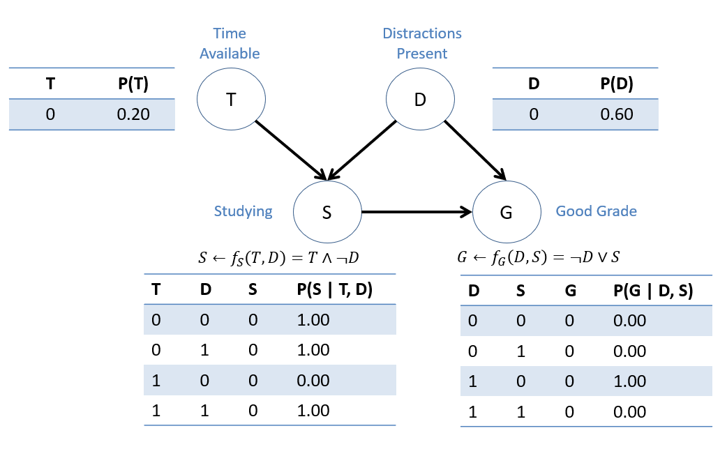
Suppose we're interested in assessing the causal effect of studying and begin by querying \(P(G=1 | do(S=0))\) (the probability of obtaining a good grade IF one were to skip studying.)
Compute \(P(G=1 | do(S=0))\) in the fully-specified SCM above.
\(P(G=1 | do(S=0)) = 0.6\). You could go through the full math of enumeration inference as practice, but we'll just logic this one out: Since \(f_G(D, S) = \not D \lor S\), if S is set to 0, then the only chance for G to be 1 is through D being 0, which happens (via the CPT on D) 0.6 of the time.
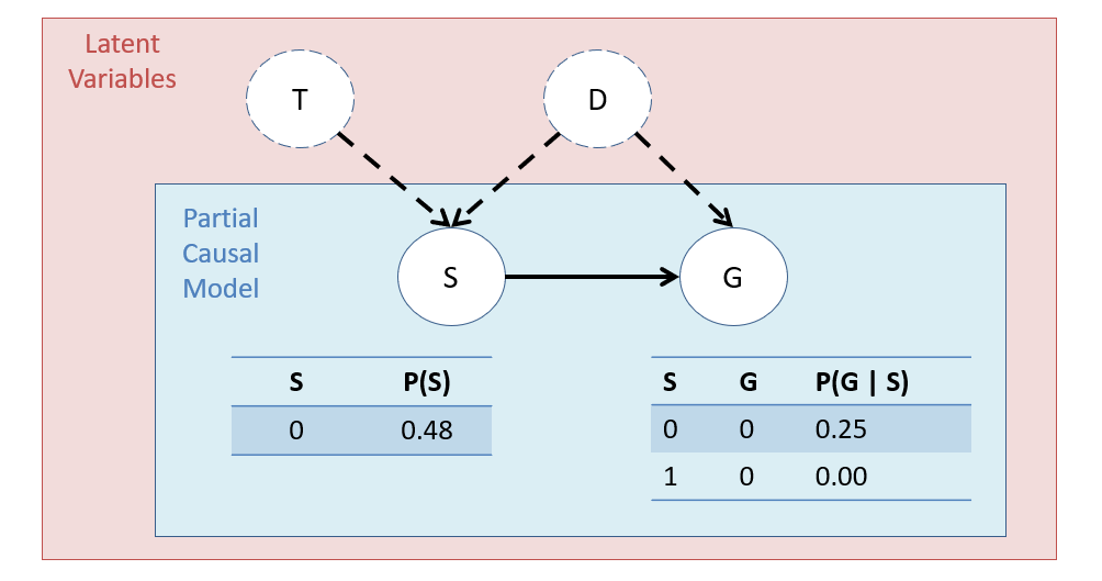
Now, suppose (due to lack of data), we fail to collect vars \(T, D\) in our dataset (i.e., they are latent), and so have only CPTs on the following partially-specified, semi-Markovian SCM; in the absence of \(T, D\), we have only CPTs on \(S, G\), whose probabilities will be summations over the latent vars.
Some things to note on the above:
This model would be an example of a semi-Markovian causal model because it has an UC \(D\) that spuriously correlates \(S\) and \(G\).
Notice the CPT row \(P(G=0 | S=0) = 0.25\) because, if \(S=0\), it could have been due to T being 0 but D still being 1 and enabling G = 1. We just don't know!
Notably, this ignorance creates an uncontrolled spurious correlation between \(S, G\) that makes the causal effect of S on G indistinguishable from the effect of the confounder's (D) effect on G.
Tangibly, this becomes problematic if we try to compute the same query as in the fully-specified SCM (wherein we *know* what the right answer should be):
Compute \(P(G=1 | do(S=0))\) in the partially-specified SCM above IF we only had access to the CPTs from our observed data on \(S, G\).
\(P(G=1 | do(S=0)) = 0.75\)... but this isn't the right answer, since we know what it should've been (0.6) in the fully-specified SCM!
So what are we to do? Throw up our hands any time some little UC comes and rains on our parade?
Of course not! (well, sometimes, but not always!)
Dealing with UCs
UC Property 1: Our models should be capable of confessing where (structurally) UCs are / may be present in the system.
Graphically, we can model UCs as additions to the structure using bi-directed dashed arrows, summarizing those that we don't know about through a confounding arc indicating unobserved, spurious (i.e., non-causal) dependence between variables.
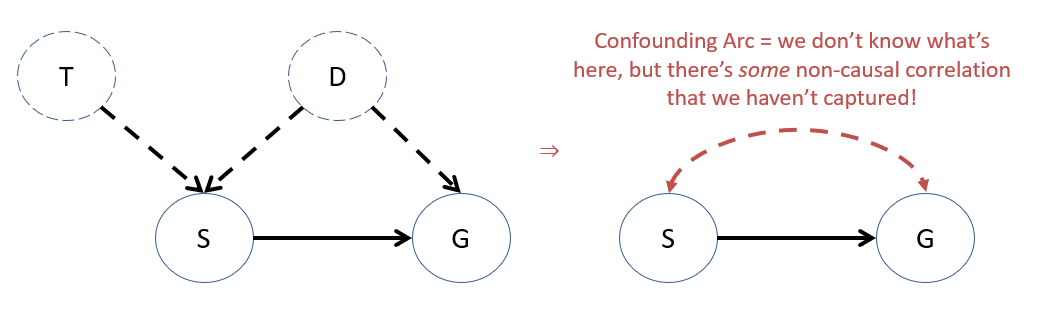
Later, these confounding arcs will be useful in determining just
UC Property 2: For the purposes of measuring accurate causal effects, we only care about latent variables that are forks to other observed variables; never sinks or chains!
Consider some system in which we are interested in the causal effect of \(X\) on \(Y\) in the presence of some latent variable \(U\):
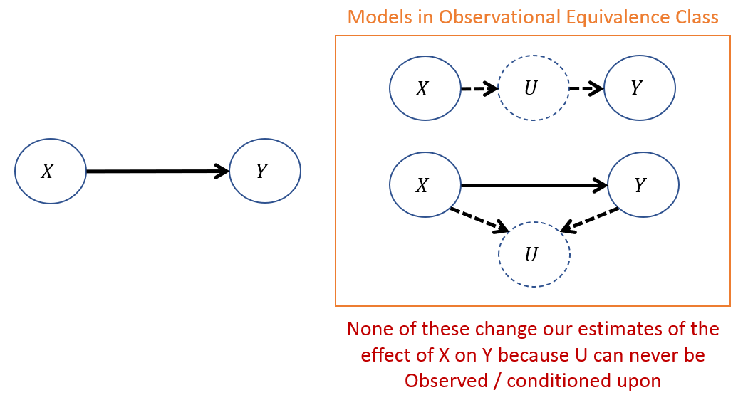
In the above models of the observational equivalence class, we see that:
With the chain \(X \rightarrow U \rightarrow Y\), X will still affect Y, just through U (indirectly), so failing to capture \(U\) in our model doesn't change anything about our predictions of X's affect on Y.
With the sink \(X \rightarrow U \leftarrow Y\), since \(U\) is unobserved, we can never condition on it, meaning it will always be a closed path through which no non-causal information flows between \(X, Y\).
UC Property 3: In Markovian models, ALL causal queries can be answered... but in semi-Markovian, some cannot be.
Why do you think Markovian models are more desirable for causal inference than are semi-Markovian?
Markovian Models are the most ideal for Causal Inference because the CPT probabilities encode latent influences that *only* affect single variables, and so no spurious / backdoor correlations are introduced between any other variables that do not carry causal information.
Some notes on the above:
Not all causal queries are contaminated by confounding! Part of the tricks in the arsenal of causal inference are to answer important questions *despite* the presence or suspected presence of UCs.
We'll need new tools / mechanics to discuss just what causal queries are estimable from the model and data we have, and the ability to both detect and account for unobserved confounding will be a prevalent future topic.
Defense of a Markovian vs. Semi-Markovian Model stems largely from the necessary condition of satisfying the Global Markov Condition AND background knowledge about the system. We'll see later tools to help defend when a model is Markovian or not.
Warning: If you're thinking: "Hey, how to determine if your model is Markovian or not?" you're not alone! A future lecture will address issues with how to detect / rule out UCs in your system.
In brief: any time we conclude that our BN is causal (a CBN), we must be able to do so on sound, scientific, and defendable grounds.
Some relationships are easier to defend than others, and we'll see later how we can go about doing so.
Identifiability and Adjustment
The setting is this: we sometimes have causal queries of interest but possess only data that may be infected by unobserved confounding, and a Semi-Markovian model that confesses *where* this confounding is believed to exist.
This adds another piece to the puzzle of our causal inference engine -- answering whether or not we can even answer a given query!
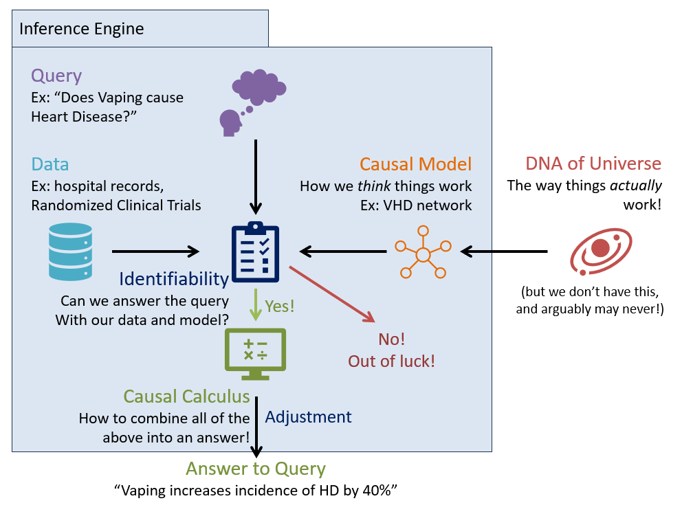
Given a causal model \(M\), a causal effect (tier-2) is said to be identifiable if it can be estimated from (possibly confounded) observational model parameters (tier-1).
Equivalently, identifiability asks, "Can we measure a query in the interventional subgraph \(G_x\) (what we want) from parameters in the un-intervened graph \(G\) (what we have)?" If the answer is "Yes," then that causal effect is identifiable.
In a Markovian Model, *all* causal queries are identifiable... only in the presence of unobserved confounders in Semi-Markovian models *might* a causal query *not* be identifiable.
To answer questions of identifiability, we'll need to define and defend 2 things:
Identifiability Criteria: which determine, given some causal graph \(G\), whether a causal query \(P(Y|do(X))\) is identifiable from observations in \(G\).
Adjustment: if a causal query *is* identifiable, provides an "adjustment formula" to compute the tier-2 query from the tier-1 data / parameters.
Let's start by intuiting some identifiability criteria.
Identifiability Intuition
Disclaimer: there are several different identifiability criteria in causal inference; we'll examine the most utile herein.
To build some intuition, consider a confounded Vaping / Heart Disease example wherein Exercise and Heart Disease have some UC.
Suppose we wish to know whether or not the causal query \(P(H = 1 | do(V = 1))\) is identifiable in this model.
This query is tantamount to asking: "Can we control for ALL spurious correlations (indicated in red below) in the model between \(H, V\) in terms of only the un-intervened model's parameters?" These spurious pathways are the non-causal ones.
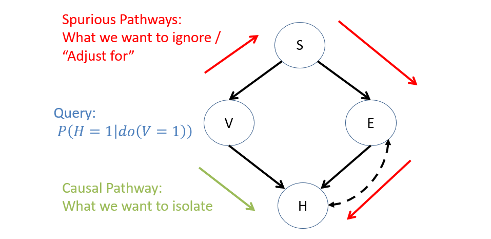
Do we have a tool (hint: think about the graph) that would could allow us to render this spurious pathway inert between our intervention variable \(V\) and our query variable \(H\)? In other words, how have we blocked the flow of information in a BN before?
How about conditioning! If we condition on \(S\), this will intercept the spurious pathway between \(V, H\) because of the rules of d-separation! Caution: conditioning on \(E\) actually will NOT work -- do you see why? The only other problem with conditioning on S: conditioning inserts its own non-causal information we'll have to account (i.e., adjust) for.
Intuition: if we can make our query \(H\) and intervention \(V\) independent in all spurious pathways *except* the causal one, then we have successfully measured / isolated the causal effect of \(V\) on \(H\).
This intuition lays the groundwork for one of the first and most useful criterial for identifiability.
Back-Door Criterion
Back-door Criterion: a sufficient (though not necessary) condition for identifiability, which says that a causal effect of \(X\) on \(Y\) is identifiable if there exists a third set of variables \(Z\) such that:
\(Z\) blocks all spurious paths between \(X\) and \(Y\): meaning that given \(Z\) blocks (by the rules of d-separation) every path between \(X\) and \(Y\) that contains an arrow into \(X\).
\(Z\) does not open any new spurious paths between \(X\) and \(Y\), which could happen if \(Z\) opens a spurious collider / sink that was not previously open.
\(Z\) leaves all directed paths from \(X\) to \(Y\) unperturbed: meaning that no variable in \(Z\) is a descendant of \(X\), lest it incorrectly intercept a portion of the causal effect of \(X\) on \(Y\).
Intuition: all components of the back-door criteria are in pursuit of isolating the causal effect of some intervention \(X\) on some query \(Y\). This means adjusting for the non-causal components in the CPTs (spurious "back-door" pathways) and leaving the causal (i.e., downstream) ones alone.
Back-door Adjustment: if such a set \(Z\) *can* be found, \(Z\) is said to be a "back-door admissible" set, and the causal effect of \(X\) on \(Y\) is given by the back-door adjustment formula: \begin{eqnarray} P(Y=y|do(X=x)) &=& \sum_{z \in Z} P(Y=y|do(X=x), Z=z) P(Z=z|do(X=x)) \\ &=& \sum_{z \in Z} P(Y=y|X=x, Z=z) P(Z=z) \\ &=& \sum_{\text{For all contexts}~z \in Z} \text{{Effect of X on Y in Context Z} * {Likelihood of Context Z}} \end{eqnarray}
Let's return to our confounded Vaping / Heart Disease example:
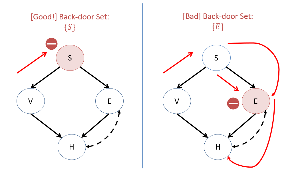
Suppose we wish to estimate \(P(H=1|do(V=1))\) from the Semi-Markovian model above, having only observational data. Is there a back-door admissible set of variables that would render this quantity identifiable, and if so, what?
Yes! \(Z = \{S\}\) (treating stress as a context in which to investigate vaping's effect on heart disease) serves as a back-door admissible set, whereas and \(Z = \{E\}\) (likewise for exercise) does NOT work, as it has an open path from \(V \leftarrow S \rightarrow E \leftrightarrow H\) with the confounding arc acting as a hidden sink between \(E \leftarrow UC \rightarrow H\).
Left as an exercise: double check that, using the rules of d-separation, why each of the sets in the answer above either do or do not work!
Visually, we see that no spurious information about \(V\) "leaks" to \(H\) through the \(Z = \{S\}\) set, but it *does* through the \(Z = \{E\}\) set:
Using the back-door adjustment formula, how would we compute \(P(H=1|do(V=1))\) using our back-door set \(Z = \{S\}\)?
Using the back-door adjustment formula where \(X = V, Y = H, Z = S\), we have: $$P(H=1|do(V=1)) = \sum_s P(H=1|V=1,S=s) P(S=s)$$
Back-Door Edge Cases
Let's think of a couple of edge cases with the back-door criterion.
Consider, once more, the confounded Smoking [S] and Lung Cancer [C] scenario debated in court with big-tobacco:
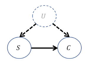
Is the causal effect \(P(C=1|do(S=1))\) identifiable in this model using the back-door criterion?
No! Here, \(U\) is unobserved, cannot be conditioned upon, and therefore, there is *no* back-door admissible set of variables that identifies the desired causal effect.
As it turns out, even though the back-door criterion is a *sufficient but not necessary* identifiability condition, there is *no method* that allows the causal query to be estimated from observational data in this scenario!
These scenarios are important because they encode that notion of honesty we talked about: the ability of our models to confess that there are some queries that we cannot answer!
Suppose we have the following causal graph for any arbitrary \(X, Y, Z\). This is sometimes called the "M-graph" setting.
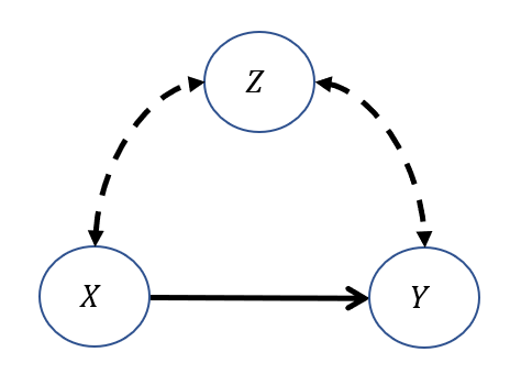
Is the causal effect \(P(Y=1|do(X=1))\) identifiable in this model using the back-door criterion?
Yes! The funny edge case: the back-door admissible set \(Z = \{\}\) is the empty-set!
Warning: if, by conditioning on a variable we *create* a spurious correlation, the causal effect will not be identifiable!
As such, in the above "m-graph," we should *not* condition on \(Z\) and so the causal effect, and application of the back-door adjustment on the empty-set, is: $$P(Y=1|do(X=1)) = P(Y=1|X=1)$$
Simple, and elegant!
Front-Door Criterion
Now the back-door criterion is a very useful tool and helps to deconfound many causal queries in Semi-Markovian models, but you might've noticed mention that it is a sufficient, though not necessary condition for identifiability.
Consider an expanded version of our Smoking / Lung Cancer example from before in which we know that the only reason \(S\) has a causal effect on \(C\) is through deposits of Lung Tar \(T\). The question: is \(P(C|do(S))\) now identifiable though it wasn't before?
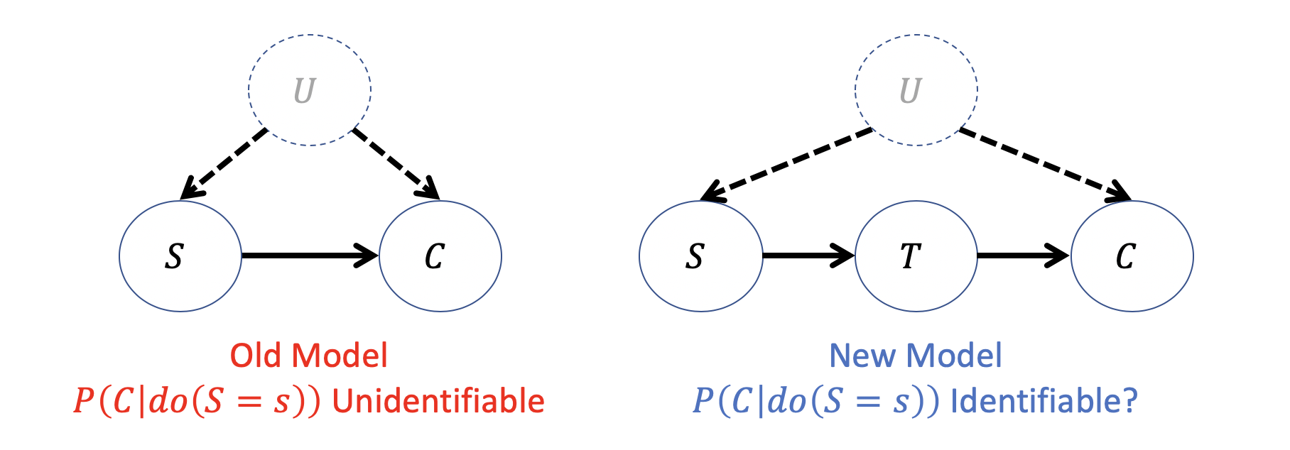
Is there a back-door admissible set to deconfound the causal effect of \(S\) on \(C\)?
No, since we cannot condition on latent variables... BUT...
What causal effects *are* identifiable in the graph?
It turns out we can identify two causal effects despite the confounding: (1) \(P(T|do(S))\) and (2) \(P(C|do(T))\).
Thank goodness these are hypothetical interventions -- I don't think any of us would care to participate in the study wherein half of us had tar forced into our lungs (oof I even cringed writing that).
How are these two effects identifiable? Well, let's think:
Note that the causal effect of \(P(T|do(S))\) is identifiable because there is a backdoor admissible set \(Z = \{\}\) -- the empty set! This is because the backdoor between \(T, S\) through \(U\) is actually blocked at the collider \(C\). As such, we have: $$P(t|do(s)) = P(t|s)$$
Now, for the causal effect of \(P(C|do(T))\), here again we have a backdoor admissible set \(Z = \{S\}\), and so can plug into our backdoor adjustment formula: $$P(c|do(t)) = \sum_s P(c|t,s)P(s)$$
With those causal effects identifiable, how might we leverage them to identify our original query \(P(C|do(S))\)?
Intuition:
There's some likelihood of seeing each value of \(T=t\) when we force \(S=s\).
For each of those values of \(T=t\), if we were to intervene on \(do(T=t)\), there's some likelihood of seeing the queried value of \(C=c\).
Solving the original \(P(c|do(s))\) just scales one by the other for each value of \(T=t\)!
Combining that wisdom symbolically, we see that:
It turns out this relationship is another adjustment formula that, unimaginatively, involves using the "Front-door" between some treatment and outcome, or in our case, the thing that separate our treatment \(S\) and outcome \(C\) through the front-door \(T\).
Front-door Criterion: a sufficient (though not necessary) condition for identifiability, which says that a causal effect of \(X\) on \(Y\) is identifiable if there exists a third set of variables \(Z\) such that:
\(Z\) intercepts all directed paths from \(X\) to \(Y\): important for establishing a causal effect of \(X\) on \(Z\) even if there is no back-door admissible set for \(X\) on \(Y\)
There is no unblocked back-door from \(X\) to \(Z\): ensuring that the effect of \(X\) on \(Z\) is not subject to any spurious correlations.
All back-door paths from \(Z\) to \(Y\) are blocked by \(X\): ensuring that the effect of \(Z\) on \(Y\) is not subject to any spurious correlations.
Front-door Adjustment: if such a set \(Z\) *can* be found, \(Z\) is said to be a "front-door admissible" set, and the causal effect of \(X\) on \(Y\) is given by the front-door adjustment formula: \begin{eqnarray} P(Y=y|do(X=x)) &=& \sum_z P(z|x) \sum_{x'} P(y|z,x')P(x') \end{eqnarray}
Note how above there is both a value \(X=x\) (the hypothesized intervention value) and \(X=x'\) (the value of the inner sum's iterator)!
And those are our two most important adjustment formulae in a nutshell -- are you feeling well adjusted?
One little caveat for those with future interest:
Both Back- and Front-Door Criteria are special cases of a more general identifiability algorithm known as do-calculus, which is a set of rules for symbolically transforming (a la, via search) expressions with do-terms to those that are do-free. If this conversion is possible, the desired effect is identifiable.
That said, do-calc is a bit out of scope for us in here, though a graduate treatment on the subject would dive much more heavily into this as it serves as a cornerstone for much of causal inference.
Hope you've enjoyed this part of the ride, kinda neat intuitions to be had all around!