Just as we examined constraint propagation as a means of improving backtracking by limiting the domains of variables, thus reducing the branching factor of the search component, we can think of a variety of additional improvements that are necessary for solving large CSPs.

[Brainstorm] Can you think of some other ways of reducing the amount of work a backtracker would be required to do for solving CSPs?

Here are a few possibilities, a couple of which we will explore today.

• k-consistency: Rather than verifying node \((k=1)\) and arc \((k=2)\) consistency, including through forward checking and constraint propagation, we could consider checking consistency between some \(k \gt 2\) node domains, and incrementally increase \(k\) until we had our original number of nodes. This does indeed describe a class of algorithms, but ones we will not examine in this course.

• Ordering Heuristics: the order in which we choose to assign to variables and the choices of values to assign during backtracking can dramatically influence the performance of the CSP solver.

• Exploiting CSP Structure: the format of a given constraint graph can lead us to some shortcuts in solving it, and identifying these becomes a huge time saver.

There are additional strategies that will take a very different approach to solving CSPs than we've been doing with backtracking, but we'll examine these in the following lecture.

For now, let's chase some of these leads down and see how we might improve our CSP solvers.

We've hinted at how the order in which we explore assignments to variables can matter, so let's now examine how and why.

Let's start this exploration with a little intuition:

What constitutes a failure during the course of backtracking / constraint propagation such that we can characterize what we would like to *avoid* during the backtracking process?

Two ways to look at it: we want to avoid making an assignment that violates a constraint, or more presciently, avoid making an assignment that shrinks the domain of a variable to the empty set.

[Intuition] So, the intuition with carefully selecting an order of assignment is to avoid catastrophically shrinking any variable's domain as early in the process as possible.

Let's look at an example and see how we can start to process this intuition.

Consider the following Constraint Graph associated with the Map Coloring problem on 6 variables with different domains.

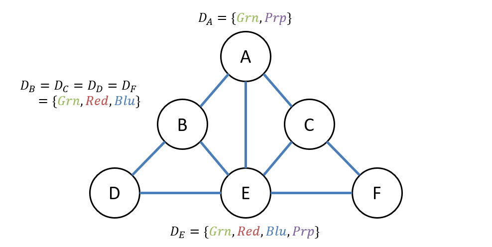
Given the choice of first assignment, which variable should we assign to first during backtracking? Why?

Assign to \(A\) first since it is the most at-risk of having no assignable values later in the process!

This is a cheap and easy heuristic to compute since we can assume having instant access to all variable domain cardinalities:

Ordering Heuristic 1 - Minimal Remaining Values (MRV): the MRV heuristic stipulates that, during backtracking, the variable with the smallest domain should have priority assignment over variables with larger ones.

This changes the backtracking algorithm from having a *FIXED* variable assignment order, to one that is dynamically chosen at every stage of the assignment.

[Reflect] Why do we want to select the variable with the *fewest* values left in its domain sooner than those with *more* values remaining?

Harken back to our intuition: we want to avoid reaching a state at which a variable has an empty domain, and there is a higher likelihood that (through assignment) we exhaust a smaller domain before a larger one.

For this reason, the MRV Heuristic is sometimes referred to as the "Most Constrained Variable" Heuristic, and ensures that any failures that would be caused by variables with smaller domains occur *sooner* in the backtracking than *later.*

The alternative is having a bunch of (albeit small) leaves in the recursion tree that do not pan out.

So, OK -- suppose we decide to start with variable \(A\) in our example above; let's consider another question...

Choosing variable \(A\), there are two values in its domain we can attempt to assign next; which should we try *first* and why?

Perhaps try Purple because it least-limits the domains of connected variables!

Ordering Heuristic 2 - Least Constraining Value (LCV): given a variable chosen for assignment, attempt to assign its values in the order of least-to-greatest values removed from other domains.

How would we assess which value of a variable is the least constraining?

This is not without cost! We would need to do forward checking (at the least) or AC-3 for each value and count the domain restrictions that amount.

There's no such thing as a free lunch!

LCV, when applied on large problems, can save an enormous amount of work, but entails doing at least one step of look-ahead to determine the impact of assigning each value!

These are the two primary order-heuristics used in concert with backtracking, but are not the only improvements we can make to CSP solvers.

Let's take a look at a separate direction next...

Thus far, we've been examining strategies that employ a CSP's constraint graph, but have not thought about how we can *exploit* key parts of that structure to improve performance.

We'll motivate these structural concerns with a CSP from the past, in which we had 3 numerical variables with a variety of numerical constraints.

[Intuition] Problems like the above require constraint propagation due to the presence of cycles in which assignments / domain restrictions to one variable may iteratively affect the others, circularly.

This may appear unavoidable in the general sense, and that perspective is not far from the truth... however, let's think about the *best* case scenario.

Consider the following 3-variable CSP constraint graph, and determine whether or not we need to consider both arcs from any two variables \((X, Y), (Y, X)\) in constraint propagation.

In the constraint graph above, do we need both directions of arcs from each connected variable during constraint propagation, or could we get away with just 1? Why?

We can get away with just 1-direction IF we assign to variables in the opposite direction, because then each assigned value will find at least 1 value that is consistent with it!

A useful property of constraint graphs without cycles: constraint propagation need be only unidirectional with assignment done in the opposite direction.

Intuiting the above: enforcing AC from \(A \rightarrow B\) ensures that when we assign to \(B\), we are *guaranteed* that *at least one* of the remaining values in \(D_A\) will be consistent with the assignment.

It turns out that this exploit doesn't apply to only linear constraint graphs, but a more general data structure...

What simpler / more restricted data structure is a graph with directed edges but without cycles?

A tree!

It turns out that tree-structured CSPs come with some nice performance guarantees when we envision the constraint graphs as trees with a root!

Exploiting Tree Structured CSPs

---

To see the utility in tree-structured CSPs, consider the following example of the Map Coloring problem with some pre-restricted domains. On the left: the original constraint graph. On the right: conceiving of this graph with \(A\) as the root.

Some things to note about the above:

• Take a moment and convince yourself that this is indeed a tree structure. It need not be a binary tree, but if you imagine picking up this graph at the chosen root \(A\) and then letting the other nodes dangle by gravity, you can see the tree structure shake out.

• This "tree-ization" of the graph is not unique! We could have just as easily have chosen \(C\) or any of the other variables to be the root so long as there are no cycles in the graph.

• Once a root is chosen, the edge directions can be chosen by a breadth-first traversal starting at said root.

Using this "tree-fied" constraint graph is now a breeze, and proceeds in two steps:

Trace this procedure through the example CSP given above!

Step 1 - Indexing: Here's an example indexing, which is not necessarily unique:

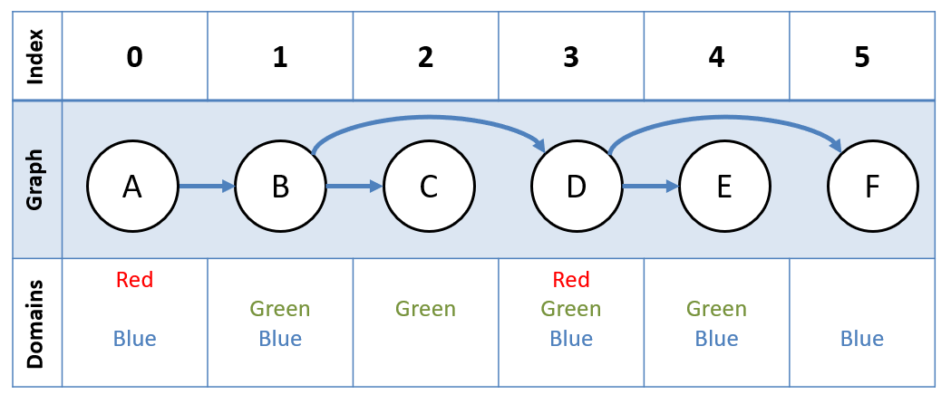
Step 2 - Bottom-up Constraint Propagation: we'll start with \(i=5\), then, for each inbound arc in descending index order, ensure arc consistency.

Step 3 - Top-down Assignment: start with \(i=0\), then, for each outbound arc in ascending index order, make an assignment that is consistent with the previous.

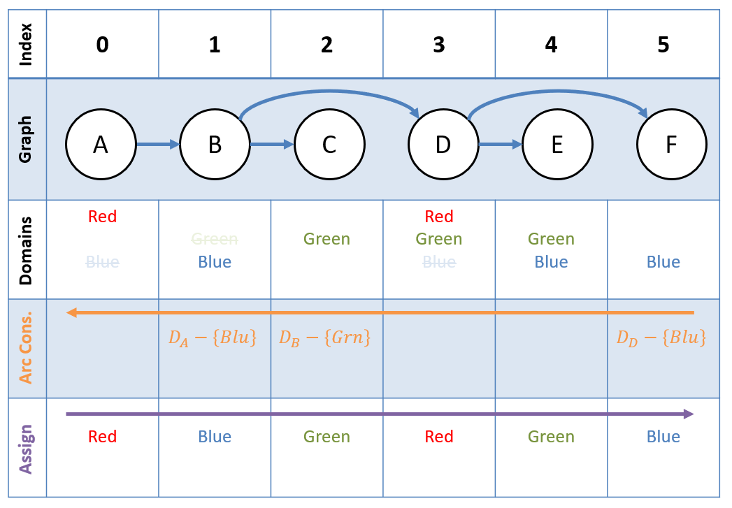
Given the procedure above, in terms of the number of variables \(n\) and the domain size of each (assuming, for simplicity, uniform domains) \(d\), what is the computational complexity of CSP solvers for tree-structured constraint graphs?

\(O(n*d^2)\), since ensuring arc consistency between any two variables is a \(d^2\) operation, and that is performed once for each of the \(n\) variables.

Neat! But, we should temper our expectations a bit:

Why is this procedure a bit of a "blue-skies" hope to have work?

It relies on the constraint graph being tree-structured, which it won't always be!

We'll address this issue, and some deeper analysis, next time!

To recap:

• Arbitrary CSPs have a solution complexity of \(O(d^n)\) due to the DFS behavior, even with heuristic improvements.

• Solving tree-structured CSPs is a much more manageable \(O(n*d^2)\), but not all CSPs are tree-structured!

Can you think of a strategy to compromise between these extremes for solving arbitrarily-structured CSPs?

Try to massage them into tree-structures!

This might work for some nearly-tree-structured CSPs, in a technique that we'll explore next.

To motivate this technique, let's see an example...

Motivating Example

---

Consider the following constraint graph and observe how it is nearly-tree-structured.

The the CSP above, how do you think we could somehow make solving this more tree-structured?

Consider variable \(E\) separately from the rest, then solve the others with \(E\) removed!

Let's see this suggestion in action; what if we considered \(E\) separately?

Note how the remaining variables are indeed in a tree-structure, and can be solved much more easily than if we were to use a naive approach.

How to go about this?

Cutset Conditioning

---

Cutset Conditioning is a technique for solving nearly-tree-structured CSPs in which some variables are assigned to separately from the rest, removed from the constraint graph, and leaving a tree-structured CSP for those remaining.

Cutsets are some set of variables that are cut (severing edges) from the original constraint graph and solved separately.

Conditioning is the process of assigning a value to some variable in a cutset, performing forward checking on its neighbor domains before cutting, and finally, severing it from the original graph.

Putting this all together, we can see how the steps of cutset conditioning unfold:

1. Step 1: Choose some cutset(s) of variables that leaves a remaining graph that is tree-structured.

2. Step 2: In traditional backtracking fashion, condition on the cutset.

3. Step 3: Solve the remaining tree-structured CSP.

Pictorially, these steps look like the following on our example above:

Things to note from the above:

• There *are* algorithms to select the cutset, but we won't be discussing those here.

• We could do this for multiple cutsets during step 1.

• For cutsets of size \(c\), the complexity becomes a very manageable \(O(\text{Solving cutset} * \text{Solving Tree-Subgraph}) = O(d^c * (n-c) * d^2)\)

• There are other structure-based CSP solvers as well, but we'll stop with cutset conditioning.

Whew! That's all there is to say about standard CSP solvers, we'll look at some more exotic techniques next time around!