Backtracking Alternatives
Let's take a quick review at the wonderful journey we've been making through the world of CSPs:
We started with naive backtracking as an adaptation to Search to solve CSPs, but these alone were computationally difficult.
We then enhanced backtracking with domain-reducing algorithms like forward checking and constraint propagation. We even enhanced it with heuristics like MRV and LCV.
We improved on backtracking's exponential computational complexity when we could coerce constraint graphs into tree-based structures.
Still, with all of these improvements, I'll pose a simple question:
With the best of these above enhancements, could we solve an N-Queens problem with \(N = 10,000,000\)?
Not tractably! That's an enormous amount of computational power that would have to go into its solution.
For reference, you can solve N-Queens with standard backtracking + heuristics in the range of \(N = [1000, 10000]\)
Can you suggest some (possibly, very different!) strategies that might be at least be able to solve these huge CSPs with a high probability?
You'll likely have a variety of (probably plausible!) suggestions here, but we're going to look at 2 over the course of the last lectures.
Find some way to randomly assign variables, and then repair that random assignment into a solution.
Identify and combine the best parts of different (failing) solutions, in an attempt to create a successful one.
We'll look at each of these fun alternatives next!
Local Search
With backtracking, the fundamental assumption was that we started with an empty assignment to variables, and then through each ply in a depth-first search, assigned values to variables to incrementally build up a solution.
Local Search is an iterative search strategy for solving CSPs (and some other problem types as well!) that is neither complete nor optimal, but can be used to find solutions to large problems when backtracking is intractable.
The steps of local search are, broadly, as follows:
Randomly assign values to each variable within their legal domain without worrying about violated constraints.
Find the set of variables with violated constraints.
Attempt to reassign to one of those variables.
Repeat until a solution is found (or you give up!).
Local search is another algorithmic paradigm that, although we'll see applied to CSPs, can also be used in a variety of different contexts.
For now, let's answer a few questions about these steps in terms of CSPs, per usual, as motivated by an example.
Motivating Example
Consider again the Republic of Forns Map Coloring problem with \(k = 3\) colors.
Step 1 - Random Variable Assignment: suppose we begin by assigning the following colors to the variables in the CSP; note: they do not form a solution, but are *close* to one.
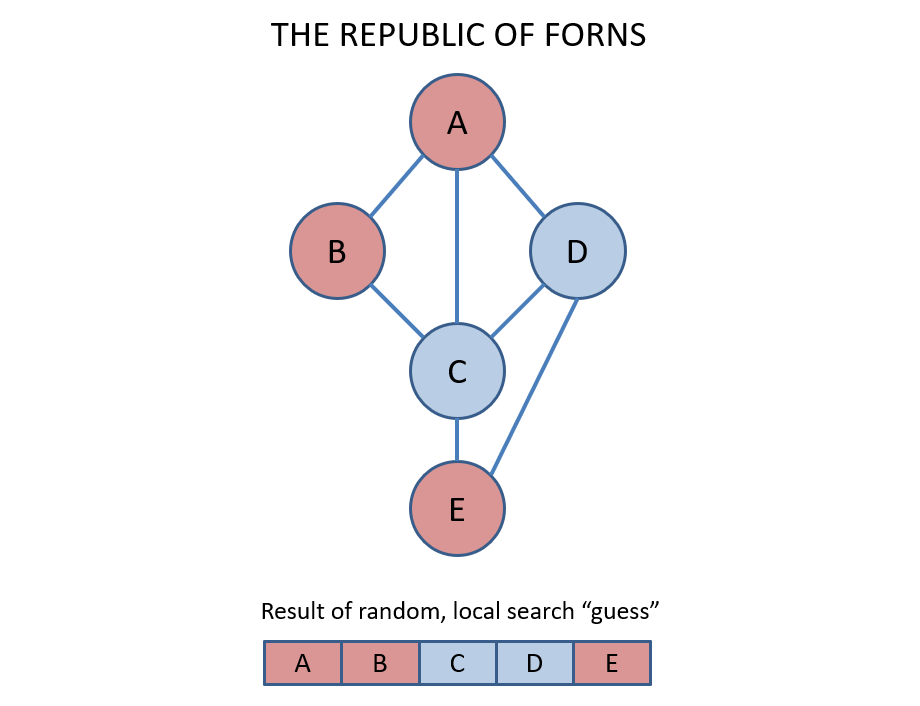
Plainly, this is not a solution, and we can see that 4 / 5 variables are in conflict with one another -- let's see if we can repair them!
Step 2 - Select a variable with a violated constraint at random.
In vanilla local search, *any* conflicted variable is chosen to be reassigned with equal probability!
Why do we choose *any* of the conflicted variables to reassign rather than, say, the one violating the most constraints?
Suppose, by reassigning the most conflicted (call this var \(A\)), we make another variable violate the same number of constraints (call this \(B\)), such that we ping-pong between assigning to \(A, B, A, B, ...\). Choosing conflicted variables at random gets us out of ruts!
In our example, we see that variables \(A, B, C, D\) have conflicts, so we'll choose \(A\) at random for the next part of the example.
Before we do, we can see what the options available to us are for each variable.
In Local Search, the set of all states that are possible from changing the value of 1 variable at a time is known as its neighborhood.
We can see the neighborhood of our Map Coloring example below:
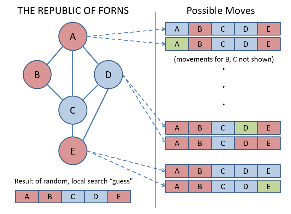
The next question to answer is: which member of the neighborhood should we visit next?
Step 3 - Reassign to the chosen conflicted variable: just how we choose the value to assign to it can be discussed next.
How we characterize the quality of a reassignment hinges on a little intuitive vocabulary:
Upward Moves reduce the number of conflicts before vs. after the reassignment.
Downward Moves increase the number of conflicts before vs. after the reassignment.
Sideways Moves keep the number of conflicts the same before as after the reassignment.
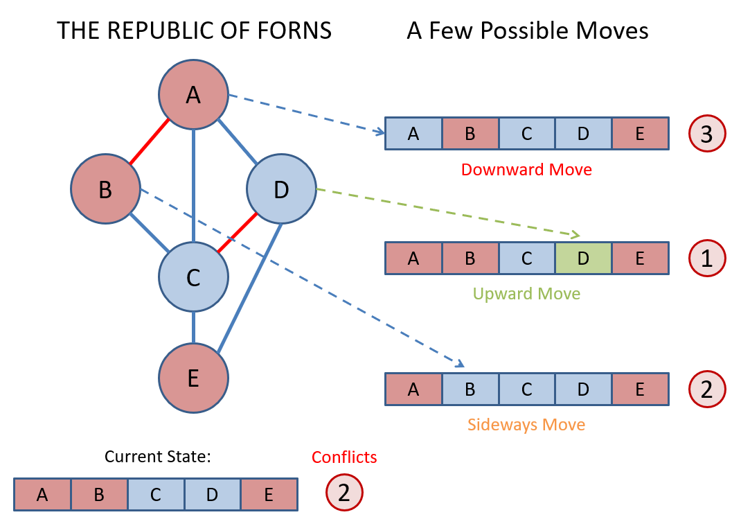
Considering our example above and that we chose to reassign to \(A\) at random, which value would be reasonable to choose? By what rule could we make that choice?
Assign \(A = Green\) because it results in the fewest number of conflicts afterwards!
The Min-Conflict Heuristic says to choose the value for a reassigned variable that results in the fewest number of residual conflicts; choose one at random in the event of a minimal tie.
Some things to note about the Min-Conflict Heuristic:
You may not get so lucky with the reassignment of a variable so as to reduce its conflicts to 0 (although we did in the case of reassigning \(A = Green\)); this is fine and expected, because we assume that in a future iteration, we'll have time to rectify that mistake.
The Min-Conflict Heuristic attempts to only make upwards / sidways moves that improve the quality of some assignment (or at least, does not damage the quality of some assignment) iteratively.
We'll see how this verbage becomes even more appropriate shortly.
However, in the meantime, we note that assigning \(A = Green\) doesn't complete our example. So, we have to repeat steps 2 and 3 until we do.
Step 4 - Repeat steps 2 and 3 until solution found.
Suppose we next chose to reassign conflicted variable \(D\), and using the Min-Conflict Heuristic, assign it a value of \(D = Red\).
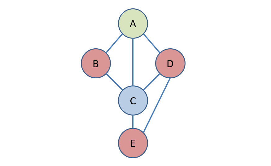
We're not done yet! We would have to finally assign a value of \(E = Green\) in a future iteration as well!
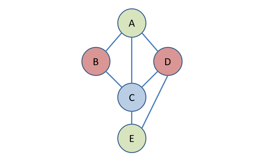
Some things to note about the procedure and example above:
We were able to find a solution with fewer assignments than there are variables! (if you don't count the original random assignment).
The result here is far from unique; we could have randomly chosen to assign to different variables in a variety of different choice points. Some choices will be more direct than others.
Local Search Characteristics
So now that we've seen Local Search in action, a few analytic questions await us:
Compared to backtracking, does local search demand more or less space / memory?
Much less! As opposed to managing a recursion tree with a potentially large call stack and many local variables allocated along the way, Local Search is an iterative solution that operates only on a single state representation.
So, from a space-efficiency standpoint, Local Search is really preferable. Managing a call stack in backtracking for large numbers of variables becomes untennable very quickly.
As for its computational analyses, the answer is less clear-cut.
Because Local Search is neither complete nor optimal, ascribing any asymptotic guarantee is out of the question.
However, *empirically,* local search tends to have near constant-time performance for even massive CSPs, except for a small case of problems!
That's an incredible pseudo-guarantee for an algorithm that isn't even complete! However, we should discuss what sorts of problems cause issues for local search.
The performance of local search depends on the ratio between the number of variables and constraints in the CSP such that: $$R = \frac{|Constraints|}{|Variables|}$$
Performance degrades sharply in a small area around what is known as the critical ratio between these two cardinalities:

Just how this critical ratio is described depends on the specific CSP being solved. However, we can still intuit why either side of it has better performance.
Why do you think performance is better on either side of the critical ratio?
Intuiting each side separately:
On the left, there are fewer constraints than variables, meaning there are likely to be fewer conflicts overall to resolve.
On the right, there are fewer variables than constraints, meaning that the variables are *so* constrained that zeroing in on the smaller solution space becomes easier.
Local Search, like many of the other topics we've touched on, has a lot of study behind it; which variables to randomly assign to, which values are best, etc. has been a topic of heuristic development for some time.
At this point, we'll take a small step back and analyze Local Search in the context of a wider class of problems and consider a troublesome issue with the above.
Hill Climbing
Now, equipped with our vocabulary, let's think about how to proceduralize a couple of ambiguous steps from the general Local Search definition above.
An objective function decides the quality of some state by a problem's specification. Sometimes called its value, a state can be evaluated by something like the min-conflict heuristic or other such heuristics.
An objective function literally defines the goal of some agent in an environment and assigns some numeric score that is higher the better some state is at satisfying that goal.
For CSPs, what would make a good objective function that, given a state (i.e., some assignment to variables), would "score" how good that assignment is?
How many / percent of constraints satisfied!
The objective, of course, is to satisfy *all* of the constraints, but that doesn't mean that certain states aren't closer to satisfying those than others.
We can plot, for some arbitrary local search map-coloring problem, the objective function for each state within their neighborhood, and observe the different components

Warning: this drawing is for intuition only and is a flattened, 2-D version of what the neighborhood of a map-coloring problem could like like; in reality, the curve would be in many dimensions that can't be drawn on the printed page!
Some parts to label above:
The current state is one that might be encountered after a random guess or after a modification of the state. Each move (a reassignment to one of the variables) can be qualified as an upward, sideways, or downard move (up the hill, across a plateau, and down the hill, respectively).
Different local search strategies are thus characterized by how they navigate the so-called "objective function hills."
Springboarding off of our min-conflict heuristic, the most basic is a greedy approach called Hillclimbing: always take the best move until you can improve no more!
  s = pick a random initial state
  while s not solution:
      n = highest value neighbor in neighborhood(s) (like by min-conflict)
      // Local maxima hit if n is not a solution:
      if n is a lower value than s:
          return s
      s = n
  return s
Yet, looking at the graph above, there's a small problem with hill-climbing approaches...
What is the issue with naive hill-climbing approaches, and can you suggest a simple fix to overcome it?
They may get stuck at a local optima! Instead, once one such local optima is reached (i.e., there are no more upward moves available to it), we can simply try again!
Hill Climbing is a lot like scaling a mountain in the fog -- you know which way is up and which is down, but you don't know if you're scaling Everest or an ant-hill.
OK, maybe that analogy's a bit dramatic, but it gets the point across...
Hill Climbing with Random Restarts is a hill climbing approach such that, whenever a local maxima is hit, and a solution is not yet found, the agent will restart from another randomly initialized state and try again.
As dumb as random restarting sounds, it can produce a solution *significantly* more often than without it.
Some other notes about random restarts:
One difficulty: it might be challenging to determine *when* we are at a local maxima vs. the global (less so in CSPs), and so it's possible to run many iterations of Hill Climbing with Random Restarts and then use the *best* of those uncovered.
This technique's chief weakness: (apart from being incomplete) it gives up very easily once it's hit a local maxima -- even if this happens to be only a few downward-moves away from a global one!
Can you propose an improvement to Hill Climbing (even with Random Restarts) that may help ammeliorate the weakness described above?
Make it willing to accept *some* downward moves, though control how likely it is to do so as the search iteration continues.
If we were to implement such a technique, would we prefer the downward moves to happen more often at the *beginning* of an attempt or near the *end?* Why?
The beginning! If we start taking a lot of downward moves near the end, we would never hit a global optima!
The whole point of "willful" downward moves is to prevent us from getting stuck at a local maxima, so taking downward moves earlier rather than later helps to un-stick us.
It turns out this technique has an analog to an idea in metalurgy known as annealing.
Simulated Annealing
Consider the following curve of some CSP's objective function, and suppose we are using local search to find a solution.

Where will most of our random starts for local search begin on this problem? What's the problem with those likely start locations?
They'll likely start on the large curves on either side of the global optima, and the problem is with the tiny dips on either side of the slope leading to a solution, which hill climbing would fail to overcome.
Idea: don't be so aloof that you're opposed to taking the occasional downward move!
If we can get unstuck at key junctures, this can enhance the power of hillclimbing at finding a solution without getting stuck.
Annealing is the process in metalurgy of heating a metal, and then gradually letting it cool to harden and temper.
Here's a pic of it in action!
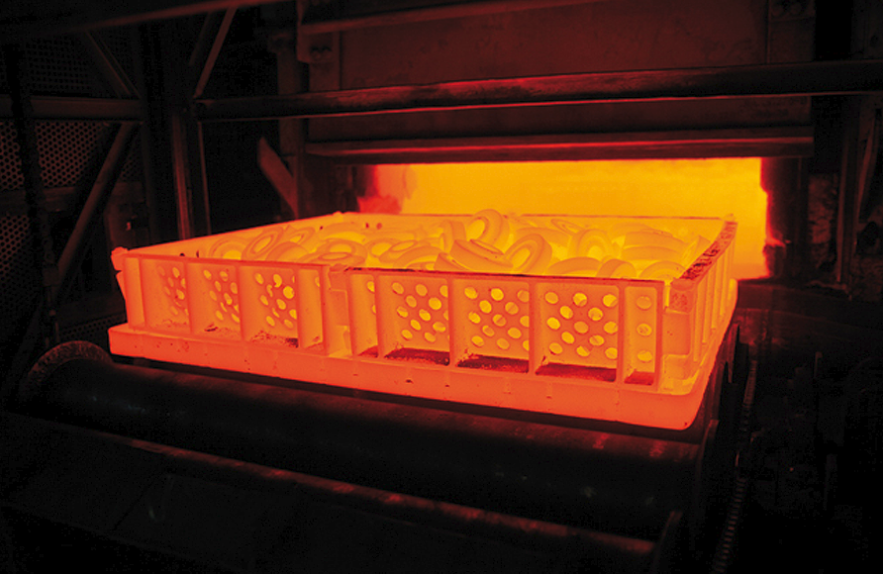
"Hold up, Andrew -- I didn't join computing for some lousy hardware concerns," you might remark... and I'm with you!
Why do you think we've suddenly started talking about annealing? What relevance does it have to our problem at-hand?
The process of gradually cooling a hot material can be analogized to having a high probability of taking downward moves while "hot," but then gradually attenuating that probability as time goes on / moves are made.
This allows us to talk not of annealing, but to instead simulate it in pursuit of improving our hill climbing!
Simulated Annealing is a programming paradigm associated with some event occurring frequently at the start of some iteration, but then decreasing over time.
There are two primary components of simulated annealing in application to enhancing Hillclimbing:
Temperature: some number that decides the probability of taking a downward move (higher = more likely).
Cooling Schedule: decides the rate at which the temperature decreases between iterations.
Simulated annealing during hillclimbing thus proceeds in several steps:
  s = pick a random initial state
  temperature = some starting temp
  while s not solution AND temperature != 0:
      n = pick a random next state in neighborhood(s)
      if n is a sideways or upwards move, move there
      if n is a downward move, only take it with some likelihood proportionate to temperature
      reduce the temperature
  return s
Without diving too much more into the idea, here's the algorithm, from your textbook:
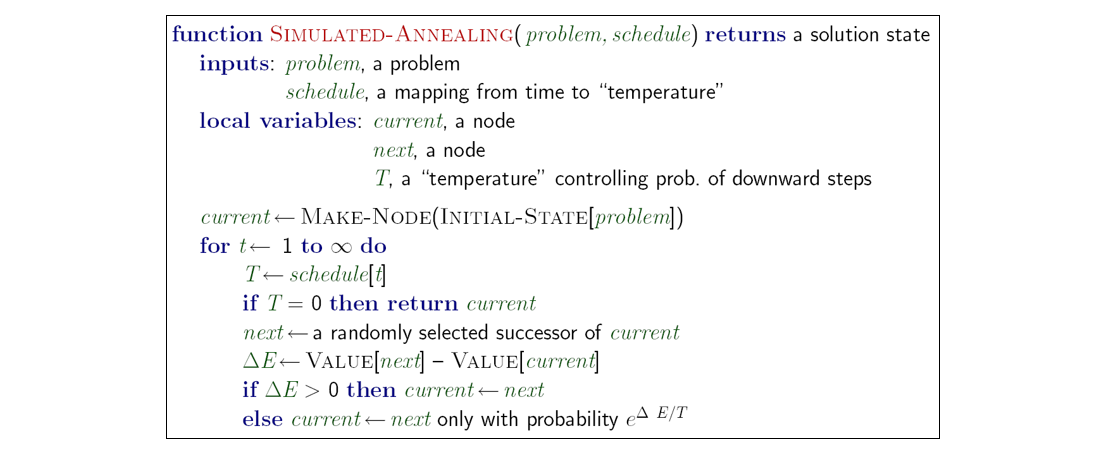
Intuitively: adding simulated annealing to your local search can help it overcome hiccups in the objective function curve that naive hillclimbing may almost never be able to solve!
Here's a visualization of simulated annealing on a more realistic 3D optimization surface but with a "flipped" objective function (lower = better). Think of this as finding the state where NO constraints are violated (i.e., all constraints are satisfied).
Notes on the above:
Each dot is another state traveled-to at a new iteration.
The color of the dot is the temperature with the red dots being hot (high likelihood of taking downward moves) and blue being cool (low likelihood).
We find the optimal solution at the end (noting once more that the "best" here is the lowest position on the surface).
Genetic Algorithms
We have one final, kinda crazy algorithmic paradigm to discuss as a backtracking alternative, and fits the bill of our somewhat probabilistic "guarantees" with local search.
One suggestion from brainstorming earlier was to consider a type of divide-and-conquer strategy, but which can still handle large numbers of variables.
Jumping to the chase, this time we're going to pull some inspiration from biology and let 'ole Mother Nature take the wheel!
Motivating Example
Consider the following two (incorrect) instantiations of the 5-Queens problem. What do we notice about them that is somewhat interesting for finding a solution?
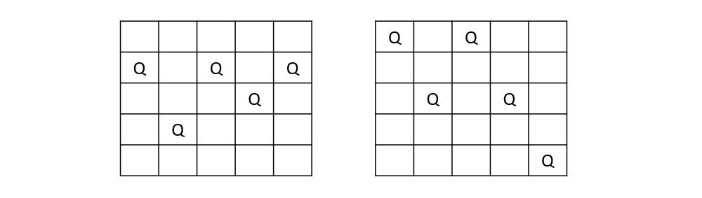
Some things to observe:
Parts of each board state are correct / conflict free, and other parts are not.
However, between the two, there exists a perfect solution (see below).
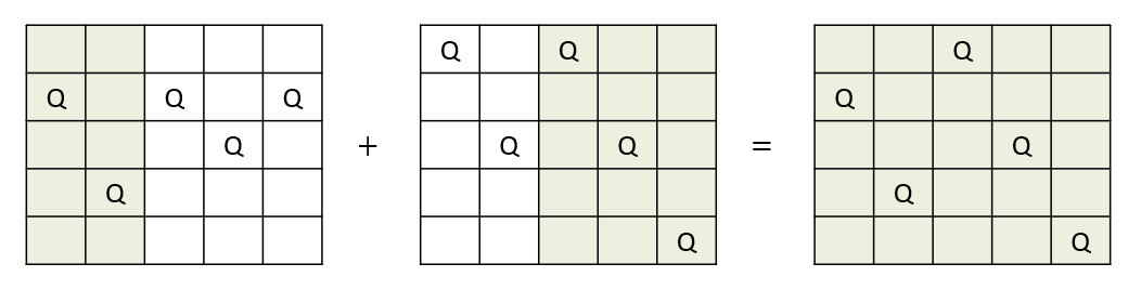
Suppose we had a strategy that attempted to take parts of two (incorrect) states in an attempt to create a new one from their pieces. What biological process does this mimic?
Evolution! Genetic recombination happens when two "mates" ... well... maybe ask your parents about what happens.
Artificial Evolution
Genetic Algorithms represent another algorithmic paradigm in which solutions can "evolve" through procedural natural selection.
Natural selection and genetic recombination are driven by, as we will apply them, some abstractions of the biological process.
The first step is being able to express the states of these problems in gene-like sequences.
Consider the N-queens problem in which, assuming each queen is placed in a different row by index in a vector, the states can be represented as vectors of column placements.
As such, consider the following representation of the 4-Queens problem in vector format:

This vector serves as *some semblance* to a genetic sequence like with nucleotides [CTGC]! With these defined, we can then
specify just how to "evolve" them into working solutions!
Genetic Algorithms are iterative (proceeding in sequential generations) until either a solution is found, or some stopping condition has been met, and are specified by several key components.
Component 1: Fitness and Selection: a Fitness Function / Score is the objective function from local search that decides the quality of a given state. A higher fitness means that it is more likely to be selected for mating.
In our N-Queens formulation, what would be a good fitness function?
How many constraints are satisfied! The more that are, the more fit that state is!
Consider the following states on the 8-queens problem in which each has a fitness score according to the number of constraints satisfied, and a selection percentage proportionate to its fitness over the total *population's* fitness.
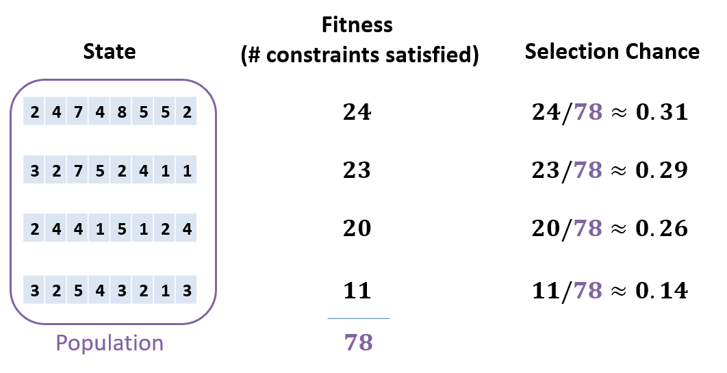
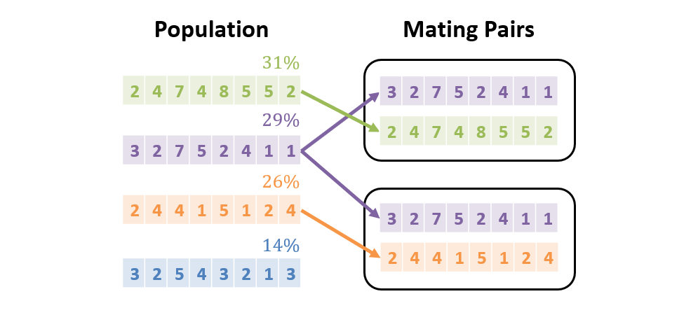
Selection: For a population of size \(N\), create \(N/2\) pairs by selecting mates based on their selection likelihood (flip an N sided-biased coin).
This means that the most fit of the population may be chosen to mate more than once, and some not at all! (though never with themselves, of course):
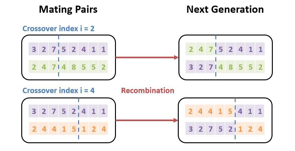
Component 2: Recombination: once mates have been chosen, new generation of "offspring" are created through a recombination of parent states / traits.
For the N-Queens problem, this can be done by choosing an index \(i\) from which each mating pair creats a pair of "crossovers" with the prop that, for parents \(P_0, P_1\), child 1 = \([P_0[0:i], P_1[i+1, n-1]]\) and child 2 = \([P_1[0:i], P_0[i+1, n-1]]\)
More clearly depicted:
Component 3: Mutation: In order to avoid getting stuck in local maxima, there is also some chance that each crossover in the new generation may have a small mutation to its "genetic" structure.
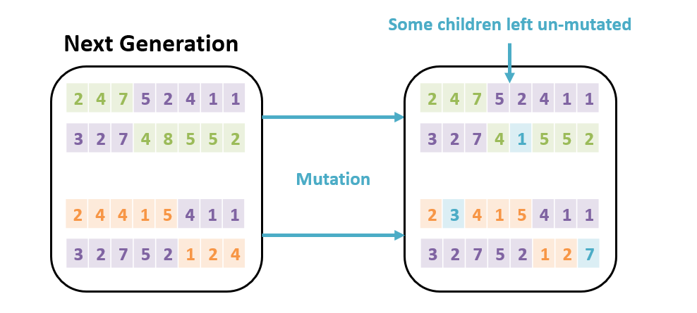
Once mutated, we have a whole new generation to test for a solution -- if none exists, we start all over again -- a story as old as humankind, literally!
Applications
This technique is neat, and in some sense, attractive (pardon the evolution pun) because of how it mimics biological processes.
Disclaimer: It is also one with only a small window of application, is often mis-applied, and satisfies a shrinking number of applications with more modern advances in AI.
Still, it can be used as a strategy for a variety of problems:
Simulating biological processes (obviously).
CSPs wherein there may be *many* local optima but few global (in which mutation can help "jump" to better problem states).
Some engineering applications, optimization problems.
Refining agents in competitive settings (literal survival of the fittest).
Generally, you're better off using Local Search or one of its variants, but there *are* some interesting explorations that use variants of these evolutionary approaches.
Some game playing agents (e.g. Google's Alpha Star) use Evolutionary Algorithms at some level of abstraction to help produce adaptive agents at large-scale games like StarCraft II! (like genetic algorithms but at a larger scale!)
Here's a fun video using genetic algorithms to make little box cars -- adorable, *and* scientific!
This, however, concludes our topics for CMSI 2130 -- you are the next generation, go forth and be fit with everything you have learned!