Assignment 1 - MAB About You

This assignment gives you some practice with Multi-Armed Bandit (MAB) problems, implementing various Action Selection Rules (ASRs), and simulating their results! Feel free to work in groups up to the group-size limit listed in the syllabus.

Here are some specifics for our simulations:

We will emulate the web-advertising click-through setting, in which the Reward Signal is binary ($Y \in \{0, 1\}$), and there are some $K$ different ads (actions, $X$) to show users. Programmatically, we will adopt a dictionary notation of {"var_name": value} to denote assignments, e.g., choosing A=1 would look like a dictionary {"A": 1}.
At each trial, the agent consults its history, chooses an ad to show (some action corresponding to the numerical index of that ad such that $A_t \in [0, K-1]$), and the environment responds with some stochastic reward, $R_t$ pulled from the simulation's arm-specific reward distribution. The agent then receives feedback pairing the action it took and the reward it received, which it then uses to update its history for the following trials.
Although the simulations are set up for scale such that arbitrary environments would allow you to make multiple decisions at a single trial and receive potentially multiple feedback variables, we will assume that there is a single decision and reward variable at each trial.
The simulation progresses over some $N = 1000$ Monte Carlo repetitions of $T = 1000$ sequential trials, in which the results of some compared agents are averaged to produce some metrics of success.
Since we are the designers of the simulation, we know (from trial 0) what the best action is (our agent, however, must learn the best action experientially), which allows us to produce some instructive graphs of how our agents are performing over time:
- Probability of Optimal Action: determines the proportion of times the agent chose the optimal action, $a^*$ at each trial. Note that this is useful because we are repeating each 1000 trial run in each of the 1000 Monte Carlo (MC) simulations, so we can get an average of when the agent learned the optimal arm choice (since on some runs it'll get unlucky and perhaps take longer to find a* than on others): \begin{eqnarray} a^* &=& argmax_a ~ P(R|a) \\ OPT(t) &=& P_t(A_t = a^*) \end{eqnarray}
- Cumulative Regret: determines the cumulative difference between the true reward expected from the optimal action, $P^*(R|a^*)$, and the reward received by the agent at time t, $R_t(a_t)$, for all trials up until $T$: $$REG(T) = \sum_{t \in T} P^*(R|a^*) - R_t(a_t)$$
  
  It might look funny having a binary value ($R_t(a_t)$) subtracted from a likelihood ($P^*(R|a^*)$) until we realize that the reward received at each trial, even if the best was chosen each time, will only pay out stochastically (that is, some proportion of the time).

Solution Skeleton

Start with the solution skeleton in-hand! Inside you'll find the directories:

GitHub Classroom Skeleton

Included in the above, you'll find:

The doc directory, in which you should place your final report.pdf containing your answers to every question.
- I suggest you compose this document using either Word with its equations editor, or LaTeX (preferably). Enumerate your answers corresponding to each problem, clearly indicating what answer corresponds to what problem!
- Your report should be single-spaced, with 1-inch margins, and at least 11pt. font (yeesh can't believe I had to write this bullet but you'd be surprised what I've gotten). Do not mail-in your answers to the questions it asks you to think about!
The main folder contains the simulation scripts described in the spec that follows.
- mab_sim.py, responsible for running the simulations and reporting the graphical results.
- mab_agent.py, responsible for defining the agent classes that will implement the ASRs that follow.
- sim_model.py, a given implementation of some Bayesian models for aiding in the simulations.
- mab_tests.py, some sample unit tests that will guide your exploration of the MAB universe.
The plots directory, containing all of the graphed metrics of success of the various ASRs following their simulation.

Before you begin the exercises that follow, I suggest you:

Create a new virtual python environment for the project (using pyenv or miniconda or the like) and then pip install the dependencies if you don't have them from past classes already, including: pip install pytest pytest-timeout mypy pgmpy pandas numpy joblib plotly (or, from within the root of the project, pip install -r requirements.txt).
Review your lecture notes for the anticipated behaviors of each ASR.
Familiarize yourself with the simulation code in mab_sim.py and ask if you have questions regarding the flow.
Familiarize yourself with the agent design stubs in mab_agent.py, in which you should plan on how to implement the agent's history, its ASR, and how to practice clean coding by exploiting inheritance to abstract commonalities (stubs given for this in skeleton).

Specifications

	GenAI use for the entirety of this assignment is BANNED for code production as it will shortcut your learning and generalizable skills (besides, there's not much code to write, the exercise is meant to teach you how to implement MAB agents from first-principles) though is always OK for understanding error messages, interpreting skeleton code, etc. as outlined in the syllabus.

It's Action Selection Rule (ASR) time! And there are a LOT of them!

We'll start with the basics and then move into some spicier environments.

The MABAgent Superclass

In mab_agent.py, implement a couple of superclass methods in MABAgent that will be used by ALL of your individual subclass agents' ASRs.

The most important in this endeavor: thinking about how to structure your agent's history.

In particular, the history should be a data structure that can be somehow used to efficiently assess action-values $Q_t(a)$.

You'll need to think about how best you wish to implement this given the following:

Actions are dictionaries mapping decision variable names (str) to their assigned values (int).
Remind yourself of how $Q_t(a)$ is computed!
Typically, to avoid issues with division by 0 for calculating $Q_t(a)$, it is safe to begin with 1 fabricated win ($Y=1$) and loss ($Y=0$) for each arm -- this puts $Q_t(a) = 0.5~\forall~a$ to start, and will be washed away with more samples as $t \rightarrow \infty$
Whatever your choice for the history, you should initialize it in the MABAgent's constructor and have a convenient means of resetting it in the clear_history method.

Once you're happy with your plan for the agent's history, continue to the next problem(s) for testing!

The Greedy Player

In mab_agent.py, implement the Greedy MAB player that, at each trial, selects the action that has the highest action-value, $Q_t(a)$.

Importantly: for any greedy choice wherein there is a tie in maximal action-value, the tie should be broken at random!

In your report, record the following:

Expectations: in a sentence or two, describe how you expect this agent to perform on the task at hand.
Sim Results:
1. Run the greedy agent unit tests via pytest -k agents_greedy
2. If all went well, you should see a graph pop up with some results and the unit tests will hopefully pass! As a reminder, all graphed results are saved in your plots directory for future reference and can be converted to an image png using the toolbox at the top right of the resulting webpage.
3. Add ALL graphs generated by these simulations to your report.

Interpretation: let's take a moment to rationalize these results.

Observe the final OPT(T=1000) value averaged over all N=1000 MC iterations and record this in the report, i.e., the average likelihood of the greedy agent discovering the optimal arm by the end of the simulation.

The simulation that was just run was with a $K=4$ arm choice MAB problem with reward distribution:

	$X=0$	$X=1$	$X=2$	$X=3$
$P(Y=1)$	0.6	0.4	0.7	0.5

From the above, we can see that arm {"X": 2} is the optimal.

In your report, in a couple of sentences, describe / derive how the OPT(T=1000) value came to be given this reward parameterization and the facts that all agents should begin with equivalent action values and ties in equivalent action values are broken at random.

The $\epsilon$-Greedy Player

In mab_agent.py, implement the $\epsilon$-Greedy MAB player that, at each trial, randomly selects some arm with probability $\epsilon$, and exploits the one it believes the best with probability $1-\epsilon$.

In your report, record the following:

Expectations: in a sentence or two, describe how you expect this agent to perform with values of $\epsilon \in \{0.02, 0.05, 0.15, 0.25\}$, i.e., which values might explore too much / too little for a time horizon $T = 1000$.
Sim Results:
1. Run the agent unit tests via pytest -k agents_epsilon_greedy
2. If all went well, you should see a graph pop up with some results and the unit tests will hopefully pass!
3. Add ALL graphs generated by these simulations to your report.
Interpretation: let's take a moment to rationalize these results.
1. Observe the final OPT(T=1000) value averaged over all N=1000 MC iterations and record this in the report, i.e., the average likelihood of this agent discovering the optimal arm by the end of the simulation for each of the agent's variants.
2. Log which agent variant ended up with the least cumulative regret--was this the same as the one with the highest OPT(T=1000)? Why or why not?

The $\epsilon$-First Player

In mab_agent.py, implement the $\epsilon$-First MAB player that randomly explores actions for the first explore_until_t trials, and forever exploits (i.e., chooses greedily) afterwards.

In your report, record the following:

Expectations: in a sentence or two, describe how you expect variants of this agent to perform with values of explore_until_t = {10, 50, 100, 200}, i.e., which values might explore too much / too little for a time horizon $T = 1000$ and the reward parameterization introduced in the Greedy agent.
Sim Results:
1. Run the agent unit tests via pytest -k agents_epsilon_first
2. If all went well, you should see a graph pop up with some results and the unit tests will hopefully pass!
3. Add ALL graphs generated by these simulations to your report.
Interpretation: let's take a moment to rationalize these results.
1. Observe the final OPT(T=1000) value for each variant averaged over all N=1000 MC iterations and record this in the report, i.e., the average likelihood of this agent discovering the optimal arm by the end of the simulation for each of the agent's variants.
2. Log which agent variant ended up with the least cumulative regret--was this the same as the one with the highest OPT(T=1000)? Why or why not?

The $\epsilon$-Decreasing Player

In mab_agent.py, implement the $\epsilon$-Decreasing MAB player that is essentially the same as $\epsilon$-Greedy, but with a value for $\epsilon$ that decreases over time by exponential decay (i.e., the exploration rate $\epsilon$ that starts at 1 and is multiplied by some decay rate at each trial).

In your report, record the following:

Expectations: in a sentence or two, describe how you expect variants of this agent to perform with values of decay_rate = {0.995, 0.992, 0.990, 0.985}, i.e., which values might cool the exploration rate too quickly / slowly for a time horizon $T = 1000$ and the reward parameterization introduced in the Greedy agent.
Sim Results:
1. Run the agent unit tests via pytest -k agents_epsilon_decreasing
2. If all went well, you should see a graph pop up with some results and the unit tests will hopefully pass!
3. Add ALL graphs generated by these simulations to your report.
Interpretation: let's take a moment to rationalize these results.
1. Observe the final OPT(T=1000) value for each variant averaged over all N=1000 MC iterations and record this in the report, i.e., the average likelihood of this agent discovering the optimal arm by the end of the simulation for each of the agent's variants.
2. Log which agent variant ended up with the least cumulative regret--was this the same as the one with the highest OPT(T=1000)? Why or why not?

The Thompson Sampling Player

In mab_agent.py, implement the Thompson Sampling (TS) MAB player, which implements a "self correcting" agent that manages exploration vs. exploitation by sampling from distributions built from the agent's history.

This one will feel a bit different than the others, as it is something of a different paradigm.

In gist, it operates as follows:

We can describe the variance associated with what we know about a particular arm's rewards through some sort of statistical distribution that we saw as a Probability Density Function (PDF).
This distribution produces some curve in which the probability mass accumulates around its average, with spread proportionate to its variance.
Sampling from this distribution is akin to throwing a dart at the curve (which is more likely to hit the larger parts of it), and using that dart's value as a noisy estimate of its value.
In the bandit setting, over time, these distributions lose variance as more samples are collected, meaning the samples will begin noisy but later converge to their "true" reward rates.

For instance, when dealing with binary rewards, we can model each arm's distribution of rewards using the Beta Distribution, which behaves as follows:

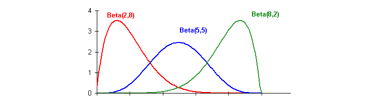
Suppose each of the above curves belongs to an arm that we have sampled 10 times:

The "shape" parameters $Beta(\alpha, \beta)$ describe how the curve appears. In application to the bandit setting, we can consider these to be (for each arm / curve) $Beta(wins, losses)$ where $wins$ means every time the reward signal was 1 in response to that chosen arm.
As such, observe the left-most, red curve: this is an arm that does not appear to be very good, as it has encountered 2 wins and 8 losses from choosing the arm associated with it. Contrast this with the right-most, green curve, associated with an arm that has experienced 8 wins and 2 losses.
Exploitation is handled such that the vast majority of "darts" thrown at the left-most curve will hit an area underneath it (with a corresponding value in the x-axis) that are less than / to the left of those that would be thrown at the right-most curve.
Exploration is handled such that there are still some chances for a dart in the left-most curve to strike it's right tail if it so happened that the dart we threw at the right-most curve struck its left tail (in the area in which they overlap).
Over time, the likelihood of exploration evaporates naturally as the probability mass centers around the true rewards.

There are tools for accomplishing this "dart throwing" in Python via the numpy.random.beta(wins, losses) method.

In a Python terminal, sample the following $Beta$ distributions associated with an arm that has a $40\%$ win-rate and then record the results in your report:

First, (what will likely be easiest as a form of clever list comprehension) obtain 10 samples from $Beta(4, 6)$. This would be the case with an infrequently sampled arm with a $40\%$ reward rate. What do you notice about the average and variance of the values that you get back?
Next, obtain another 10 samples from the same arm, but after it has been chosen more, i.e., obtain 10 samples from $Beta(40, 60)$. Reflect once more: what do you notice about the average and variance of values you get back?

In summary, the steps of Thompson Sampling are:

Obtain the beta distribution's parameters (alpha and beta = wins and losses = +1 rew and +0 rew for each arm) define what the distribution looks like and is a function of the agent's current history, $H_t$.
When it comes time to make a new choice, $A_t$, get a sample from each arm's different beta distribution, call that sample $\hat{Q}_t(a)$.
Pull the arm / choose the action with the highest sampled $\hat{Q}_t(a)$, i.e., $$A_t = argmax_a~\hat{Q}_t(a)$$
Update the history to record the pulled arm and its associated outcome, i.e., $$H_{t+1} \leftarrow (A_t, R_t)$$

Thus, over time, your history gets saturated with more samples, the corresponding beta distribution to each arm a better / less variant estimate of its true reward rate, which leads it to learn over time what the best action is!

Your challenge: take the information you learned from above to design a MAB-playing agent whose decisions are based on samples from these $Beta$ distributions.

In your report, record the following:

Expectations: in a sentence or two / pseudocode, describe how you implemented your Thompson Sampling bandit player.
Sim Results:
1. Run the agent unit tests via pytest -k agents_thompson
2. If all went well, you should see a graph pop up with some results and the unit tests will hopefully pass!
3. Add ALL graphs generated by these simulations to your report.
Sim Comparison:
Now that you've verified your Thompson Sampler, let's run a comparison on the different ASRs and see how they stack up! Execute pytest -k agents_comparison
Reflect: how did these approaches compare? Comment on the strengths of your Thompson Sampler as it might perform vs. the others if you did *not know* or did *not have* a *finite* time horizon, $T$.

They Grow Up So Fast

Now that you've had a *sample* of some bandit strategies, it's time for you to branch out a bit on your own and create your own agent!

Given all of your implementations and experience from above, create your own MAB ASR that manages exploration and exploitation in the Custom_Agent class in the skeleton!

Some rules and regulations:

Your implementation should be a creative, nontrivial ASR that uses some history to manage exploration vs. exploitation. If in doubt, ping me on Slack!
Optionally, you may implement a MAB player that you've researched but that we did not cover in class, such as the Upper-Confidence-Bound variants.

A simple UCB variant says to select arm $A_t$ at trial $t$ by the ASR: $$A_t = argmax_a~ \left[ Q_t(a) + c * \sqrt{\frac{log(t)}{N_t(a)}} \right]$$ ...where $Q_t(a)$ is the value function, $N_t(a)$ is the number of times action $a$ has been chosen, and $c$ is a hyperparameter in $[0, \infty]$ that controls the level of exploration. Higher values of $c$ means that the agent will explore more, and closer to 0 it will explore less. Experiment with and plot some different values of $c$ if you choose to implement UCB for this problem.
Your agent cannot use any between-Monte-Carlo simulation information just like the others couldn't -- no cheating!
Lastly, your agent must be specialized to this particular learning environment such that it outperforms the Thompson Sampler in cumulative regret.

After implementing this agent, log the following in your report:

Expectations: in a sentence or two / pseudocode, describe how you implemented your custom bandit player.
Sim Results:
1. Run the agent unit tests via pytest -k agents_custom
2. If all went well, you should see a graph pop up with some results and the unit tests will hopefully pass!
3. Add ALL graphs generated by these simulations to your report.

The Contextual Bandit Player

Contextual Bandit Problems are just like those we've been discussing but with one twist: before making a choice, the agent is served some number of contexts / covariates that are features related to the particular decision it must make.

Let's state some assumptions and then tackle some theoretic insights:

We must redefine the optimal *contextual* action (OPTC) as a function of some set of variables $C$ that provide maximal information about the state of the reward, $R$ (i.e., set $C$ includes all non-action variables that provide information about $R$, i.e., are dependent on it): \begin{eqnarray} a^*_{c} &=& argmax_{a}~ P(R|a, c) \\ OPTC(t) &=& P_t(A_t = a^*_{c}) \end{eqnarray}

Warning: we'll revisit this definition after the causal inference section; it actually has a bit of a subtle flaw to it that we don't yet have the tools to fix!

The flow of any one trial $t$ is diagrammed below; notice how the context is unaffected by the action, which is what distinguishes this type of problem from the changing state of a Markov Decision Process.

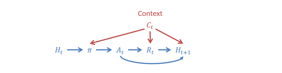
In writing, the steps accomplished at each simulation trial are:

The environment first generates any context variables c_t that will be sent to all agents in the simulation. Imagine that these are demographic info about the user you're about to advertise to like Age, Location.
Each agent generates its action choice a_t *as a function of* that context c_t
The environment responds with a reward that is function of BOTH a_t, c_t
The agent then receives feedback on its choice and the full outcome by way of a triplet {a_t, c_t, r_t}

Your task: (intentionally left as a rather open-ended one): implement the ContextualBanditAgent that takes these context variables into consideration!

In your report, record the following:

Expectations: in a sentence or two / pseudocode, describe how (1) you implemented your contextual player, (2) how it would perform against agents that do *not* take contexts into consideration, and (3) how you plan to handle the context variables in your policy.
Sim Results:
1. Run the agent unit tests via pytest -k agents_context
2. If all went well, you should see TWO graphs pop up with some results in both a simple and more complex contextual setting... and the unit tests will hopefully pass!
3. Add ALL graphs generated by these simulations to your report.
Sim Comparison:
In the "basic" contextual setting there is only a single context variable compared to the "advanced" setting that has four. What do you notice about your agent's performance between these two settings? How does the number of contexts seem to matter?

Doing Your Own Exploration

Finally, some guided outside exploration...

Last Task: Research and summarize a bandit-problem variant and a strategy used to address its unique properties.

Complete the following steps, logging each in your report -- this section should take up *no less than* half a page:

Find a MAB problem variant that you find interesting; the Wiki page on MABs lists many with resources attached.
In your own words, summarize this MAB variant and how it differs from the traditional MAB formalization above.
In your own words, summarize one of the strategies that addresses this variant's unique challenges.
Provide an example of where this variant and accompanying strategy could be applied to a task in your particular domain of computing interest.

Whew! Hope that was a fun one for ya. Next time, we'll look at the exploration / exploitation dilemma in relation to MDPs!

Submission

You will be submitting your assignments through GitHub Classroom!

What

Complete all requested sections of your ./src/mab_agent.py and ./doc/report.pdf (making sure to clearly label problem numbers and answers).

How

To clone this assignment (if you need a refresher), consult the guide here:

GitHub Classroom Tutorial

To submit this assignment:

Simply push your final, submission copy to the GitHub Classroom repository associated with your account.
Place your name at the top of *all* submitted files AND in the accompanying readme file.