Announcements
TBD!
Tree Basics
Hey, remember doubly linked lists?
Yeah me neither... well that's OK, here's a refresher:
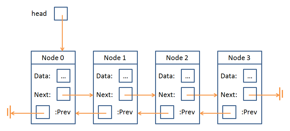
Double linked lists consisted of a sequence of nodes with data elements and pointers to the previous and next node in the sequence.
Indeed, the concept of a Node is something that Trees and Linked Lists have in common:
A Node is just an object that stores some data as well as a means of accessing other Nodes in the data structure.
The "means of accessing other Nodes" from a Node in a Linked List was to traverse it via prev and next; for Trees, it's only slightly more complicated.
Trees (in the general definition) possess Nodes with any number of "children," which are pointers to the next Node in the Tree.
Let's go over some definitions, see a Tree, and then run some code!
A Tree is yet another abstract data type consisting of data nodes arranged hierarchically, with a root node possessing some number of pointers (edges) to other children nodes, who in turn have their own children, etc.
There are two primary constraints for a Tree to be a... Tree: (1) no node's pointer (edge) points to the root, and (2) no two pointers point to the same node.
To formalize some of those definitions:
The root of a tree is a single node that has no inbound edges.
A leaf node is one that has no outbound edges.
An internal node has both inbound and outbound edges.
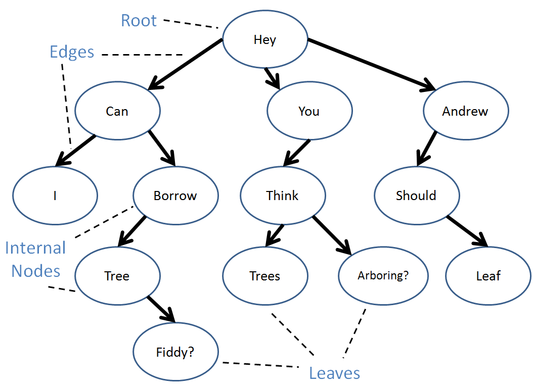
A tree can have duplicate values in its data nodes.
There are also a variety of relationships we can define between nodes:
An edge extends from a parent to a child with the arrow pointing to the child.
An path is any set of connected, directed edges.
A descendant of a node A is any node B with a directed path from A to B.
An ancestor of a node B is any node A with a directed path from A to B.
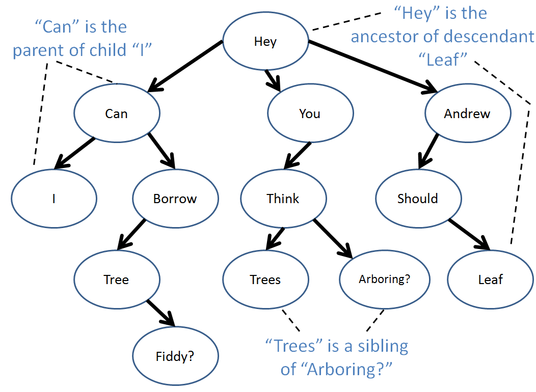

The depth of a node is equal to the number of edges along the path that separate it and the root.
The tree-depth a given tree is equal to maximum depth of any node in the tree.

Well, those are the tree basics! Let's look at some code now...
Tree Algorithms
I hope you liked recursion because trees were built for it! (or from it? any who...)
Let's start off with how we might construct a Node class:
  struct TreeNode {
      int data;
      TreeNode(int d) {data = d;}
      void addChild (TreeNode* c) {
          this->children.push_back(c);
      }
      vector<TreeNode*> children;
  };
Here, we have our TreeNode with an int data member and then an STL vector with TreeNode pointers to all of that TreeNode's children.
Let's reformat our tree from before with numerical values.

Now, let's say I wanted to create this tree using my new TreeNode class... since my numbers are conveniently in sequence, I can make a vector with them and then create the edges!
  int main () {
      vector<TreeNode> tree;
      int nodes = 13;

      // Create the TreeNodes in the tree
      for (int i = 0; i < 13; i++) {
          tree.push_back(TreeNode(i));
      }

      // Connect the nodes with edges!
      // (obviously there's a better way to do
      // this that we'll discuss next time)
      // [!] Left branch
      tree[0].addChild(&tree[7]);
      tree[7].addChild(&tree[2]);
      tree[7].addChild(&tree[10]);
      tree[10].addChild(&tree[5]);
      tree[5].addChild(&tree[4]);

      // [!] Middle branch
      tree[0].addChild(&tree[6]);
      tree[6].addChild(&tree[3]);
      tree[3].addChild(&tree[8]);
      tree[3].addChild(&tree[11]);

      // [!] Right branch
      tree[0].addChild(&tree[12]);
      tree[12].addChild(&tree[1]);
      tree[1].addChild(&tree[9]);

      // ...
  }
Now, before we dive head-first into Tree algorithms, we should always be on the lookout for these 4 test cases:
Does my algorithm work (read: not break) for an input nullptr?
Does my algorithm work for an input root node?
Does my algorithm work for an input interior node?
Does my algorithm work for an input leaf node?
Let's start off light with the following problem... which might look a little familiar:
  // Returns the maximum data node value in the
  // tree; expect no input nullptr
  int maxInTree (TreeNode* n) {
      // Set the current max to the input node's
      // data member
      int currentMax = n->data;

      // Find the max of each child's subtree
      for (int i = 0; i < n->children.size(); i++) {
          // Set currentMax equal to the max of
          // child i's subtree
          currentMax = max(currentMax, maxInTree(n->children[i]));
      }
      return currentMax;
  }
Not too bad... let's try one ourselves:
Modify your maxInTree function to implement treeDepth, a function that determines the tree depth of the input tree (TreeNode pointer).
  int treeDepth (TreeNode* n) {
      int currentMax = 0;
      for (int i = 0; i < n->children.size(); i++) {
          currentMax = ??? ;
      }
      return currentMax;
  }
Implement the nodesAtLevel function, which returns the number of nodes located at the depth specified.
  int nodesAtLevel (TreeNode* n, int level) {
      // Base case! Return when...
      if ( ??? ) {
          return ???;
      }

      // Iterate through every child
      int nodes = 0;
      for (int i = 0; i < n->children.size(); i++) {
          // [!] Add the number of nodes at the next level
          // if that's our target level! (hint: don't
          // need to use a conditional due to our base case)
          nodes += ???;
      }
      return nodes;
  }
Cool! How about a question to round things off?
Are all doubly linked lists also trees?
No! Linked lists allow for the possibility of cycles.
N-ary Trees
Whereas with the general definition of a tree allowed us to specify an arbitrary number of children for any node, there may be some benefits in restricting that number...
An n-ary tree is a tree in which each node can have at most n children.
Thus, a binary tree has nodes with at most 2 children, a trinary tree has nodes with at most 3 children... etc.
For the purposes of this discussion, we'll be examining binary trees.
Hey! Here comes one now!
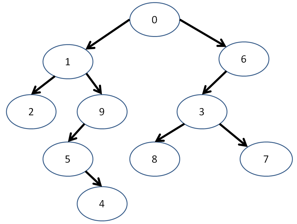
"Hey... isn't that just the last example but with the right branch gone and a couple of numbers swi--"
It's 3:00am! Sue me!
Now, the Node structure that we define for binary trees might look a tiny bit different, just by convention because we like to define "left" and "right" children.
  struct BinTreeNode {
      int data;
      BinTreeNode* left;
      BinTreeNode* right;
      BinTreeNode(int d) {
          data = d;
          left = nullptr;
          right = nullptr;
      }
  };
Again representing our example from above:
  int main () {
      vector<BinTreeNode> tree;
      int nodes = 10;

      // Create the TreeNodes in the tree
      for (int i = 0; i < nodes; i++) {
          tree.push_back(BinTreeNode(i));
      }

      // Connect the nodes with edges!
      // (obviously there's a better way to do
      // this that we'll discuss next time)
      // [!] Left branch
      tree[0].left = &tree[1];
      tree[1].left = &tree[2];
      tree[1].right = &tree[9];
      tree[9].left = &tree[5];
      tree[5].right = &tree[4];

      // [!] Right branch
      tree[0].right = &tree[6];
      tree[6].left = &tree[3];
      tree[3].left = &tree[8];
      tree[3].right = &tree[7];

      // ...
  }
Let's look at some neat properties of binary trees.
Tree Traversal
Tree traversal determines the order in which we visit each node in a tree, starting at some node (usually the root).
Traversal strategies are defined recursively, in terms of the current node, its left child, and its right child.
There are three primary traversal strategies under the heading of "Depth first" which we'll talk about later:
Pre-order Traversal
The preorder traversal strategy follows these steps:
Visit the current node (base case)
Visit the left subtree (recursive case)
Visit the right subtree (recursive case)
The definition of "visit" will depend on your application. For the moment, let's consider our application to be simply to print out the data at each Node in a given order.
  // Prints the data in each node using
  // the preorder traversal strategy
  void preorderPrint (BinTreeNode* n) {
      if (n == nullptr) {return;}
      cout << n->data << endl;
      preorderPrint(n->left);
      preorderPrint(n->right);
  }
Preorder traversal looks like this:
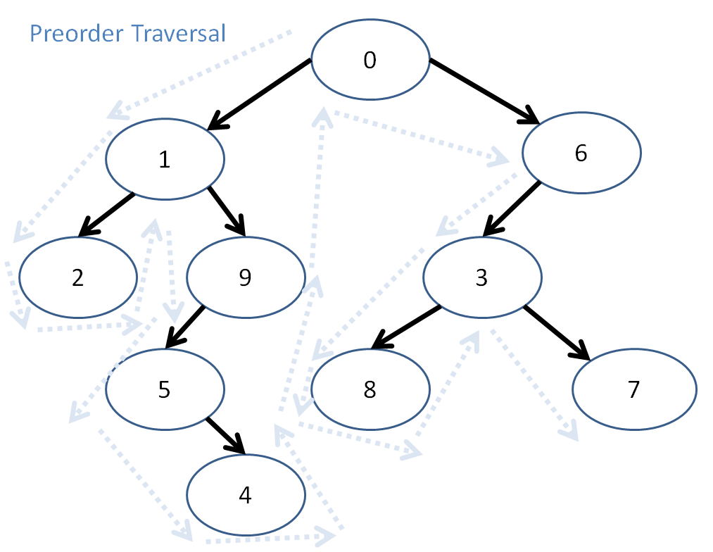
So, here, preorder traversal prints out: 0, 1, 2, 9, 5, 4, 6, 3, 8, 7
Post-order Traversal
The postorder traversal strategy follows these steps:
Visit the left subtree (recursive case)
Visit the right subtree (recursive case)
Visit the current node (base case)
NOTE: This means, even though we might "pass through" a node, we don't print it until its left and right subtrees have been processed!
Here is the postorderPrint function:
  void postorderPrint (BinTreeNode* n) {
      if (n == nullptr) {return;}
      postorderPrint(n->left);
      postorderPrint(n->right);
      cout << n->data << endl;
  }
So, what will the postorder traversal of our tree print out?
The postorder traversal prints...
2, 4, 5, 9, 1, 8, 7, 3, 6, 0
In-order Traversal
The inorder traversal strategy follows these steps:
Visit the left subtree (recursive case)
Visit the current node (base case)
Visit the right subtree (recursive case)
For completion, here's that in code form:
  void inorderPrint (BinTreeNode* n) {
      if (n == nullptr) {return;}
      inorderPrint(n->left);
      cout << n->data << endl;
      inorderPrint(n->right);
  }
Applications for Binary Trees
We've already discussed one of the most prevalent applications for binary trees: binary search.
A binary search tree is a binary tree in which all elements in the left subtree of a node are less than the data member of that node, and all elements of the right subtree are greater than the data member of that node.
Some other constraints for binary search trees is that there must be no duplicate nodes, and the left and right subtrees of each node must also be a binary search tree.
Let's revise our ongoing example:

We observe that, for each node, the left subtree contains data elements strictly less than the data element of the subtree root, and vice versa for the right subtrees.
Now, binary search becomes a trivial algorithm:
  bool binarySearch (BinTreeNode* n, int query) {
      if (n == nullptr) {return false;}
      if (n->data == query) {return true;}
      else if (query < n->data) {
          return binarySearch(n->left, query);
      } else {
        return binarySearch(n->right, query);
      }
  }
Practice Problems
Provide two binary trees that could elicit the preorder traversal print out: 5, 3, 1, 2, 0
Is it possible for a binary search tree to have the postorder traversal print out of: 12, 18, 14, 21, 20, 17
No! The 18 wedged between the 12 and 14 implies that a number greater than the root (which we know must be 17 because it was printed last) existed on the side intended to be less than the root.
Binary Search Tree Algorithms
Suppose we wish to create a binary search tree class... recall that BSTs must adhere to two principle restrictions:
No node may have more than 2 children
All nodes to the left of a given node must be less than that node, and all nodes to the right of a given node must be less than (or equal) to it
Here's a simple binary search tree class skeleton:
  struct BST {
      // BSTNode struct internal
      // to the BST
      struct BSTNode {
          int data;
          BSTNode* left;
          BSTNode* right;
          BSTNode(int d) {
              data = d;
              left = nullptr;
              right = nullptr;
          }
      };

      // Root just points to a single
      // BSTNode
      BSTNode* root;

      BST() {
          root = nullptr;
      }
      ~BST() {}; // TODO!
      bool find (int query, BSTNode* n = root); // TODO!
      void insert (int i); // TODO!
      void clear(BSTNode* subtree); // TODO!
  };
Let's start using this simple BST class by fleshing out some of its member functions!
Now, the insertion algorithm isn't too bad... let's try to code an iterative version.
Complete the BST insert function started below:
  // Creates a new node with the given data member
  // in the BST
  void BST::insert (int data) {
      BSTNode* b = root;

      // Base case: tree is empty
      if ( ??? ) {
          ???
          return;
      }

      // Otherwise, find its proper position
      while (true) {
          // Case: Data is less than current node
          if (data < b->data) {
              // If there's already a node left...
              if (b->left) {
                  // Then continue down the tree
                  ???

              // Otherwise, no node to left, so insert:
              } else {
                  ???
                  return;
              }

          // Case: Data is greater than / equal to node
          } else {
              if (b->right) {
                  ???
              } else {
                  ???
                  return;
              }
          }
      }
  }
Cool, nice and simple... we can confirm that everything's working with the following main function:
  int main () {
      BST bs; // hehe... bs
      bs.insert(5);
      bs.insert(4);
      bs.insert(6);
      bs.insert(3);

      cout << bs.root->data << endl;             // 5
      cout << bs.root->left->data << endl;       // 4
      cout << bs.root->right->data << endl;      // 6
      cout << bs.root->left->left->data << endl; // 3
  }
What is the time complexity of this insertion operation?
Finding the location to insert takes log(n) time and then the actual insertion is constant, giving us a grand total of log(n).
Now that we have a taste for building our binary search trees, we see that implementing the actual search operation is pretty simple!
We'll do things recursively this time for extra practice.
Implement the BST's find member function, which takes in a query int to find in the tree, and returns true iff that value exists somewhere in the tree.
  bool BST::find (int query, BSTNode* n) {
      // If our given node pointer is nullptr, return
      // false -- we're out of tree to examine!
      if (n == nullptr) {return false;}

      // [!] Otherwise, if the current node's data is our
      // query, we're done!
      if ( ??? ) { ??? }

      // [!] If it's not, we have to determine whether we
      // want to continue by searching the left or right
      // subtree:
      else if ( ??? ) {
          return ???;
      } else {
          return ???;
      }
  }
On average, What is the time complexity of this search algorithm? (we'll think about worst-case later)
O(log(n)), since at every step, we reduce the number of possible locations for the query to exist by about 1/2.
Great! So we've got our BSTs insertable and searchable, but what about cleanup?
Taking a step back for some review... remind me what postorder traversal is again? What's the postorder traversal of this tree?
Interesting property about postorder traversal... what happens when I remove each Node found in postorder traversal, in the order in which I visit them?
We remove each node's children before removing it! Perfect for destroying our tree nodes when we need to clean up.
So, here's a good practice problem... how might we code the destructor of our BST?
Complete the destructor helper-function code skeleton for our BST class below:
  // Clears all nodes, making sure to
  // deallocate appropriately
  void BST::clear(BSTNode* subtree) {
      // Base case: reached an ending
      if ( ??? ) {
          return;
      }

      // Otherwise, traverse and delete:
      ???
      ???

      // [!] Printout for example before
      // deleting:
      cout << subtree->data << endl;
      ???
  }

  // Destructor properly calls clear
  BST::~BST() {
      clear(root);
  }
What is the time complexity of this destruction operation?
O(n), since we visit every element once.
Binary Search Tree Node Deletion
We'll discuss how to perform arbitrary node deletion here, but won't code it (left as an exercise? yada yada).
The steps for deletion are simple.
Suppose I wish to remove node N from a BST. This removal breaks down into several cases.
Node N is a leaf: remove N, and update the parent's pointer to it to nullptr.
Node N has 1 child: update the parent's pointer to N to now refer to N's sole child, then remove N.
Node N has 2 children: replace N with the smallest element of N's right subtree (call this S), remove N, then recursively call erase on S.
We can try this operation on our favorite example BST:
Delete 12 in the above BST.
Delete 11 in the above BST.
Delete 21 in the above BST.
Balancing Binary Search Trees
Say I'm inserting ints into a binary search tree. What property of this input list of ints will cause insertion to take O(n) time?
When the insertions are done one at a time and arrive in sorted order.
Suppose I do create a binary search tree using the above detrimental insertion ordering. What efficiency guarantee on what operations does my BST lose?
I lose log(n) performance of search and insertion!
You can test out insertion into a binary tree here (click me)
Well, as it turned out, that worst case insertion was problematic... and the more linear, and less tree-like binary search trees became, the less efficient their search became too!
So the eggheads of yore considered making an algorithm that would keep the tree balanced such that any insertion won't make the tree become too linear.
Balancing binary search trees is an operation that prevents them from becoming too linear, thus securing the performance guarantees we expect in a BST.
There are a variety of different ways to keep trees balanced and maintain the log(n) search guarantee for binary search trees; we'll examine a couple now.
AVL Trees
AVL trees have 1 property in addition to those of binary search trees: the heights (depths) of any two of a given node's subtrees must differ by *at most* 1.
This enforced property makes sure that the depth of any subtree never becomes too linear, which would degrade the efficiency of search and further insertions.
This balancing act takes O(log(n)) time, which means that, upon insertion of any new value, we get O(log(n) + log(n)) = O(log(n)) time; a greater overhead, but same complexity class.
Firstly, we keep track of a "balance factor" at each node which is equal to:
balance = height(left_subtree) - height(right_subtree)A tree is out of balance if its balance factor is greater than or equal to 2, or less than or equal to -2.
If a tree is out of balance, then we use the following balancing algorithm:
  // Code skeleton for C++, edited from Wikipedia :)
  if (balance_factor(L) == 2) { // The left subtree
      Node* P = left_child(L);
      if (balance_factor(P) == -1) { // The "Left Right Case"
          rotate_left(P); // Reduce to "Left Left Case"
      }
      // The Left Left Case
      rotate_right(L);

  } else { // balance_factor(L) == -2, the right subtree
      Node* P=right_child(L);
      if (balance_factor(P) == 1) { //The "Right Left Case"
         rotate_right(P); // Reduce to "Right Right Case"
      }
      // The Right Right Case
      rotate_left(L);
  }
So what does it mean to "rotate" a tree, you might ask?
A rotation promotes a child node to the parent, and demotes the parent to a child node depending on the direction of the rotation. Subtree structures are maintained.
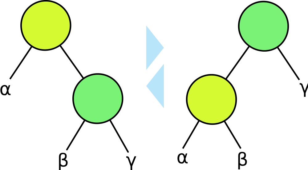
Above, a right / clockwise rotation would start at the right image and finish with the left image.
Similarly, a left / counter-clockwise rotation would start at the left image and finish with the right image.
Notice that the subtree structures are maintained with each rotation.
What would a left rotation of the 10 node look like in the following tree?
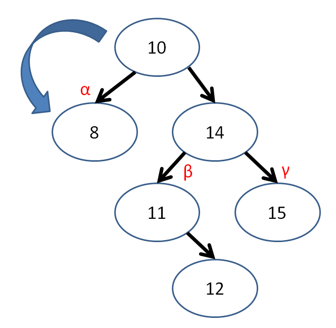
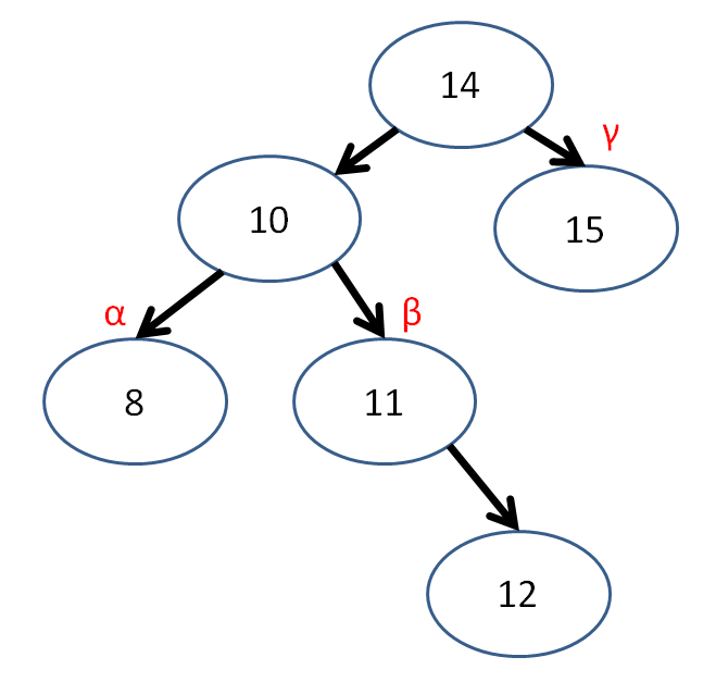
Now that we have the basics of rotation down, let's look at an example inserting into an AVL tree:

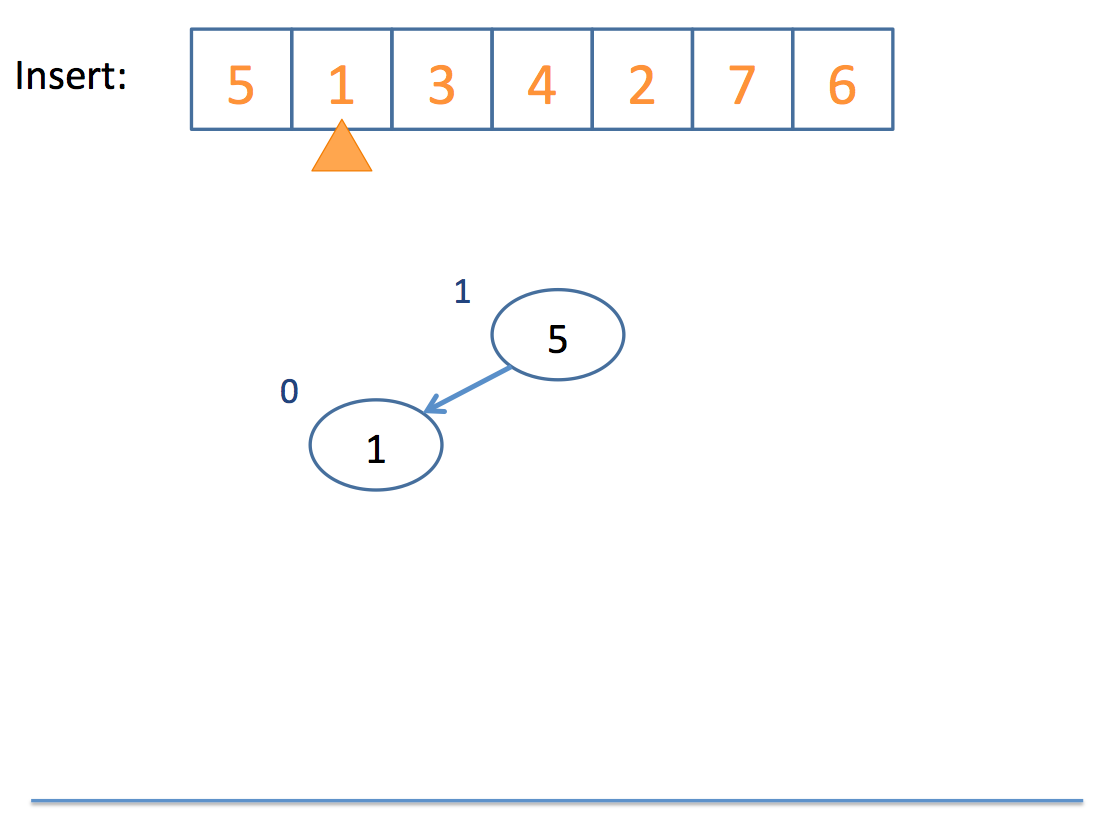
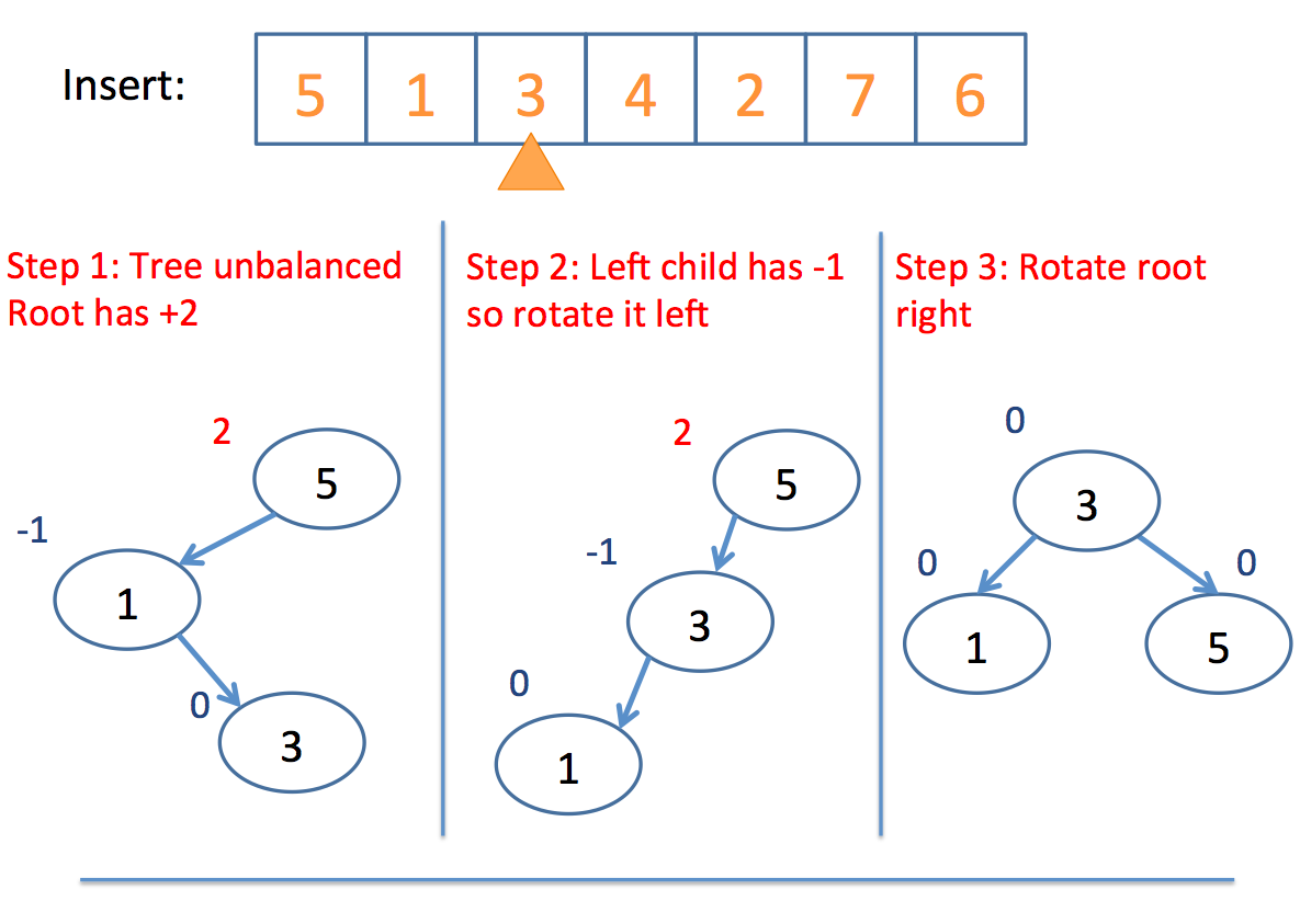

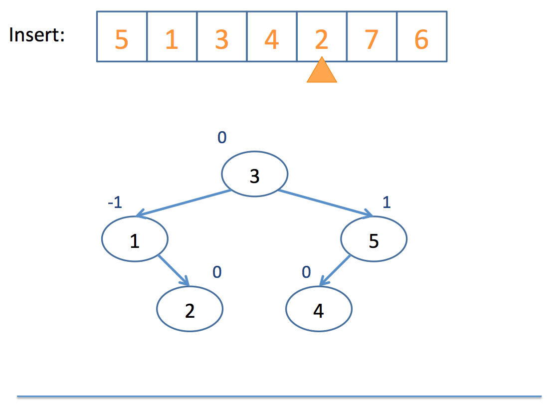
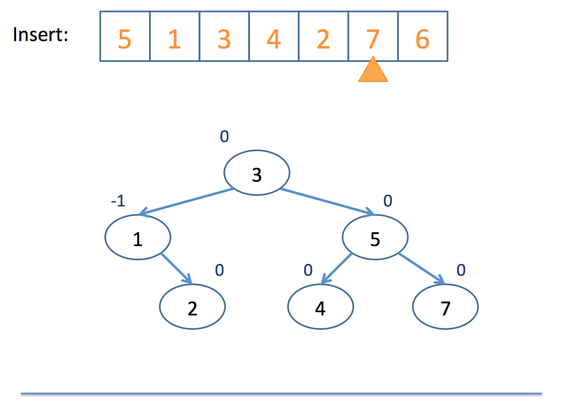
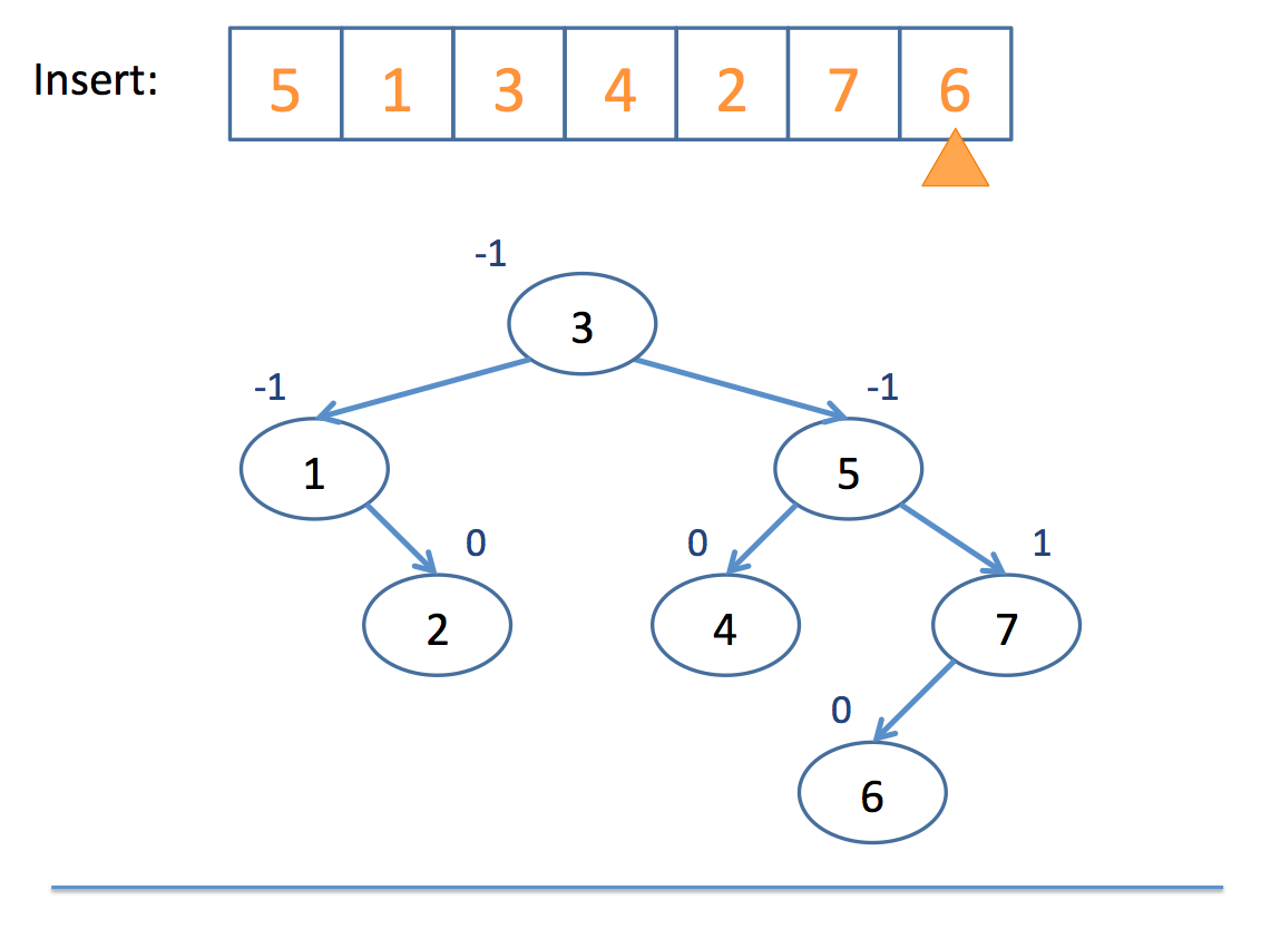
Neat!
So remember: AVL trees balance subtree heights, not necessarily just the number of nodes per subtree!
Let's examine a visualization here (click me)
Red-Black Trees
So, the one problem with AVL trees is that with a lot of insertions, you'll have to keep performing the balancing overhead any time a branch becomes 2 depths or more greater than a parent.
Red-Black Trees said, "Hey, let's not do all of this rebalancing nonsense all the time; everything's chill until the path from the root to the farthest leaf is no more than twice the distance from the root to the closest leaf."
So, without diving deep into how it rebalances when this distance is exceeded, let's just look at some properties of red-black trees lifted from wikipedia:
A node is "painted" either red or black
The root is black
Every red node must have two black child nodes
Every path from a given node to any of its descendant leaves contains the same number of black nodes.
What we end up with is a binary search tree that still ensures O(log(n)) search without the need to so frequently rebalance.
Let's examine a visualization here (click me)
Hash Tables
If you're me and you're looking for something at a supermarket, you'll probably wander aimlessly, looking at each row until you find it.
Yet, if you ask a store employee, you'll find that, for the most part, they'll know exactly which row your item is in without having to look!
(I, of course, never ask because male ego, etc.)
Now to bring the analogy home, it'd be nice if we had some "store employee" with our data structure collections that could tell tell us where to look for a query.
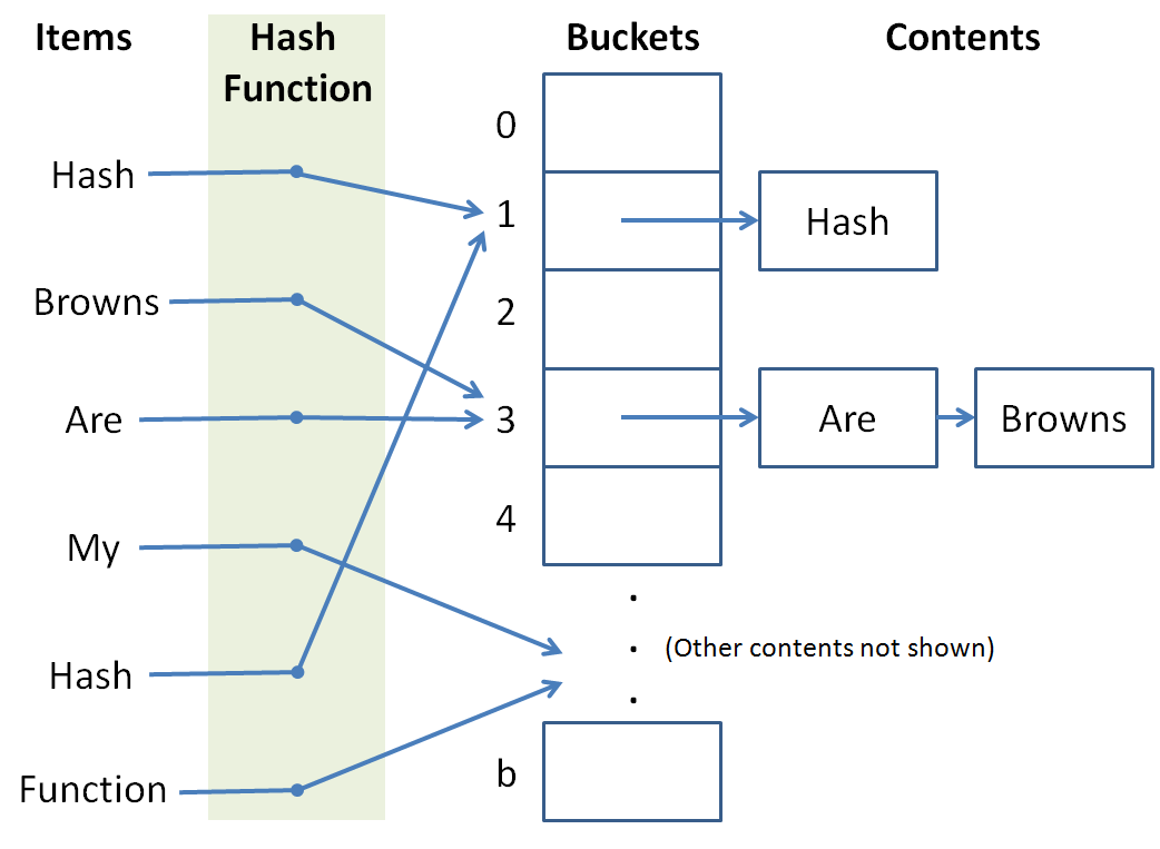
A hash table provides us with a means of storing data structures into certain buckets such that we can consult a hash function to determine where a particular item should go (for insertion) or where it might already live (for search).
For a given value to store or a query to a hash table, the hash function tells us which bucket to store it in / look in.
So, to unpack those definitions a bit:
The hash table is like the grocery store in our analogy.
The hash function is like the employee that we ask which aisle a particular item is in that we're looking for.
The hash buckets are like the aisles of the grocery store.
So why is this useful?
Well, if we had about 1000 items we needed to store, and 1000 buckets in which to store them, then assuming we chose a good hash function to evenly divide up the items into buckets, we could perform insertion and search in near constant time! O(1), wow!
This is because we reduce the possible set of matches down to only those contents of a particular bucket, which is, if the items are uniformly distributed, going to be very small compared to the original collection.
Constant time is the gold standard of data structures and you're saying it's possible?! Let us learn of these wonderous devices by building a simple one of our own.
The Hash Table
Let's begin by designing our hash table.
A hash table needs buckets that are accessible by index.
Why do our hash buckets need to be accessible by index, and what data structure what you suggest to use for our buckets?
If we want constant time lookup and search, we'll need random access or else we'd have to traverse some number of Node-like objects to reach our goal bucket. Also, it's convenient for a hash function to only hash items to integer ids. So, for the purposes of this example, we'll use a vector.
OK, let's define our HashTable class below:
  template <typename T>
  class HashTable {
      private:
          // LOL "BUCKET LIST"
          vector<list<T>> buckets;
  };
Well that's dull so far...
Note we use (for this example) a vector for the buckets (enable random access) and lists for the individual bucket contents.
We'll template our HashTable so we can store different stuff.
Now, for the constructor, how many buckets do we want to start it off with?
What is the tradeoff for having more or fewer buckets in our hash table?
More buckets means that fewer items will be in each bucket (if our hash function performs a uniform distribution of the items) at the cost of having to take up more space in memory.
So, let's start off at, say, 1,000 buckets.
  template <typename T>
  class HashTable {
      private:
          int MAX_BUCKETS;
          vector<list<T>> buckets;
      public:
          HashTable (): MAX_BUCKETS(1000) {
              // Start off the buckets with MAX_BUCKETS
              buckets.resize(MAX_BUCKETS);
          }
  };
Alright, the stage is set... let's talk about hash functions.
Hash Functions
Hash functions act as our "oracles" that tell us which bucket a particular item should go in.
They receive as input whatever item we're trying to store or lookup and output an int index somewhere between [0, b), where b is the number of buckets.
There are some properties of hash functions we need to satisfy...
Hash functions need to be fast!
If our hash function crawls wikipedia for articles on obscure topics, converts every character in those articles to its character code equivalent, adds them, and then mods them by the biggest prime number that will fit things neatly into our buckets... we're probably gonna have a bad time (literally).
So, we want something that's simple, quick, and satisfies this other property:
Hash functions need to evenly distribute our items into buckets.
If our buckets start to hold too many items, then the hash table will be pretty useless... we'll just have a linear search internal to our lists!
So, we need to determine a way to, pretty uniquely, determine what item goes into what bucket!
When a hash function maps inputs to the same bucket, we call that a collision.
Generally, we want to avoid collisions because they hurt.
But seriously, the more collisions we have, the more our complexity suffers because it means we have to find values within our lists.
A last property our hash functions should have:
Hash functions should be deterministic, meaning that if value A maps to bucket B in one call to our hash function, then it should map to bucket B in future calls as well.
Keeping this in mind, let's propose a couple of hash functions for our HashTable.
Judge whether or not the following is a good hash function:
  unsigned int hash (int toHash) {
      return toHash % 2;
  }
Judge whether or not the following is a good hash function:
  unsigned int hash (string toHash) {
      unsigned int result = 0;
      for (int i = 0; i < toHash.length(); i++) {
          result += toHash[i];
      }
      return result % rand();
  }
Judge whether or not the following is a good hash function:
  unsigned int hash (string toHash) {
      unsigned int result = 0;
      for (int i = 0; i < toHash.length(); i++) {
          result = result * 101 + toHash[i];
      }
      return result % MAX_BUCKETS;
  }
This last one isn't bad; it's deterministic, simple, and stays in the range of our max number of buckets.
Why did I choose to multiply by 101? What is special about the number 101 (or numbers like it)?
It's prime! When we multiply by a prime number, the chances of getting a unique result are higher because of the lack of factors. This helps us distribute keys to our buckets.
Alright, so let's add that to our HashTable!
We'll make it private because for this example, only our HashTable functions will care about the hash.
  template <typename T>
  class HashTable {
      private:
          int MAX_BUCKETS;
          vector<list<T>> buckets;

          // NOTE: If we want to be able to handle other
          // template types than strings for T, we'd need
          // other, more generalized hash functions...
          unsigned int hash (string toHash) {
              unsigned int result = 0;
              for (int i = 0; i < toHash.length(); i++) {
                  result = result * 101 + toHash[i];
              }
              return result % MAX_BUCKETS;
          }

      public:
          HashTable (): MAX_BUCKETS(1000) {
              // Start off the buckets with MAX_BUCKETS
              buckets.resize(MAX_BUCKETS);
          }
  };
It's coming along!
Let's examine inserting items into our HashTable.
HashTable Insertion
So now that we have our hash function and our buckets with their lists, let's define our insertion behavior.
Complete the HashTable's insertion function below:
  void insert (T toInsert) {
    // [!] Push toInsert to the back of the list that the
    // hash function gives you from input toInsert
    buckets[ ??? ].push_back(toInsert);
  }
Warning! The above insert function is missing something? What is it?
OK we'll deal with that in a moment...
I'll provide you with a neat print function just to display some syntactic sugaring for a printout:
  void print () {
      for (int i = 0; i < buckets.size(); i++) {
          list<T>::iterator it = buckets[i].begin();
          if (buckets[i].empty()) {
              continue;
          }
          cout << "=== Bucket[ " << i << " ] ===" << endl;
          while (it != buckets[i].end()) {
              cout << *it++ << endl;
          }
      }
  }
OK, so now we have the following HashTable class and a nice little test script:
  template <typename T>
  class HashTable {
      private:
          int MAX_BUCKETS;
          vector<list<T>> buckets;

          unsigned int hash (string toHash) {
              unsigned int result = 0;
              for (int i = 0; i < toHash.length(); i++) {
                  result = result * 101 + toHash[i];
              }
              return result % MAX_BUCKETS;
          }

      public:
          HashTable (): MAX_BUCKETS(1000) {
              buckets.resize(MAX_BUCKETS);
          }
          void insert (T toInsert) {
              buckets[HashTable::hash(toInsert)].push_back(toInsert);
          }
          void print () {
              for (int i = 0; i < buckets.size(); i++) {
                  typename list<T>::iterator it = buckets[i].begin();
                  if (buckets[i].empty()) {
                      continue;
                  }
                  cout << "=== Bucket[ " << i << " ] ===" << endl;
                  while (it != buckets[i].end()) {
                      cout << *it++ << endl;
                  }
              }
          }
  };

  int main () {
      HashTable<string> hashy;
      hashy.insert("To");
      hashy.insert("Hash");
      hashy.insert("Or");
      hashy.insert("Not");
      hashy.insert("To");
      hashy.insert("Hash");
      hashy.print();
  }
Now, the issue with our insert is that it currently allows for duplicate keys... we can't have this behavior in a hash table because it would be ambiguous to talk about a key (which is meant to be unique) when there are multiple instances of that key.
Let's implement our hasKey function below:
NOTE: If we were really designing a HashTable class, we'd probably want to implement a HashTable iterator, but since this is an intro example, we'll reduce the find functionality to just a boolean return function.
  bool hasKey (T query) {
      // Store a pointer to the bucket's list
      list<T>* lPtr = &buckets[hash(query)];
      // Start an iterator at it's beginning
      list<T>::iterator it = lPtr->begin();
      // Search linearly for the query item
      while (it != lPtr->end()) {
          if (*it == query) {
              break;
          }
          it++;
      }
      // Return whether the iterator found a
      // match or not
      return it != lPtr->end();
  }
Now, we can fix our insertion function to not add duplicates!
  void insert (T toInsert) {
      if (hasKey(toInsert)) {
          return;
      }
      buckets[HashTable::hash(toInsert)].push_back(toInsert);
  }
Now if we run our previous test main function, we see that duplicate keys are not added, just as we'd like. Cool!
Hash Table Complexities
So it might be clear how we're able to find a bucket in constant time (random access of vector + hash function), but why is searching the bucket list considered average case constant?
Well let's look at a certain property of hash tables:
The load factor of a hash table is the ratio of the number of items stored in total divided by the number of buckets.
So, the lower the load factor, and assuming our hash function is doing a good job of evenly distributing keys across buckets, the faster our lookup in each list is going to be!
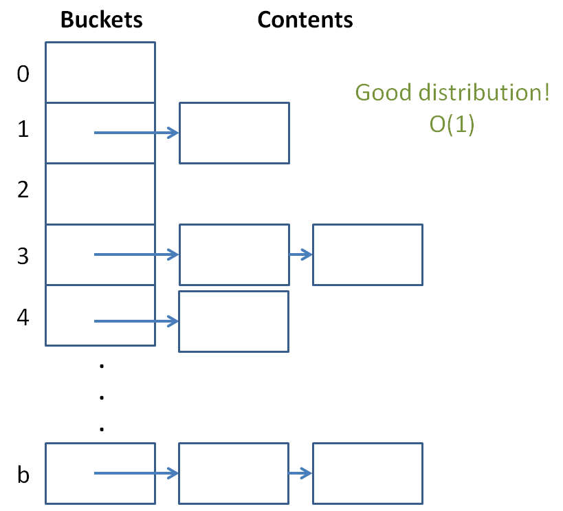
We see that a hash table with a ton of items and few buckets will have a large load factor and nearing linear lookup and insertion time.
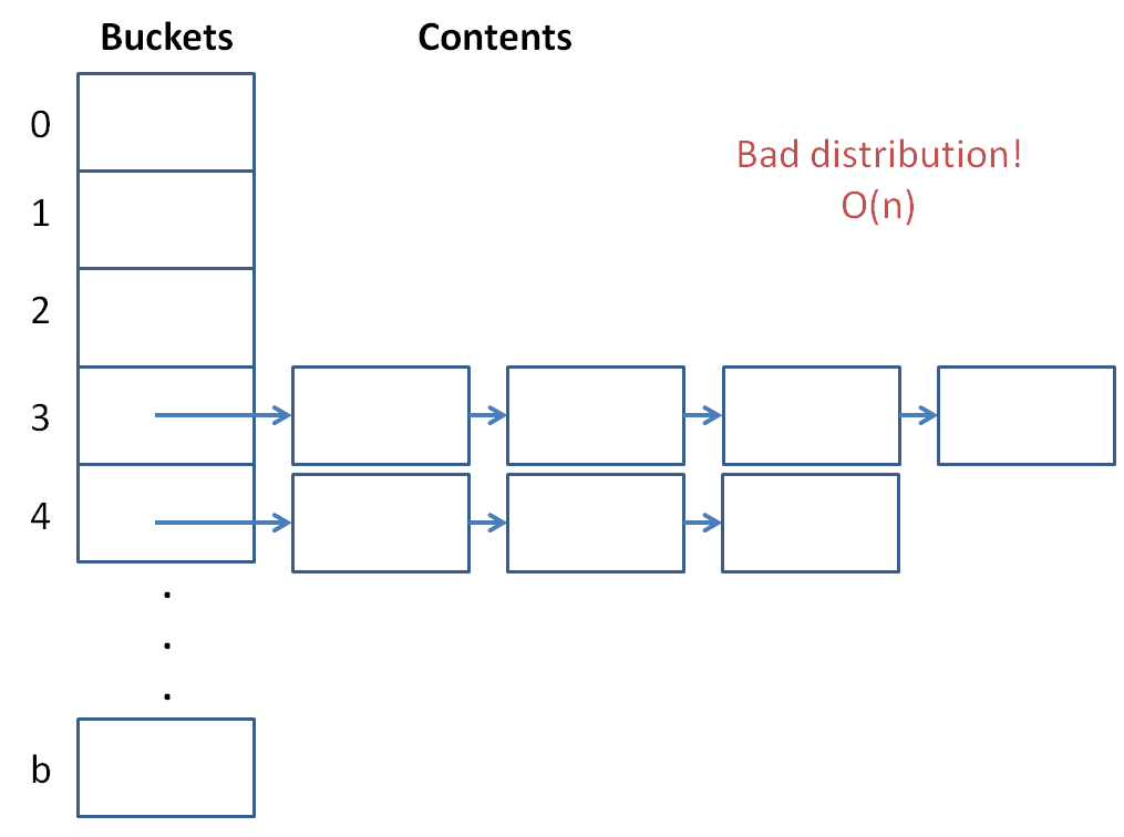
Solutions to resolving collisions depend on how we've modeled our Hashtables.
In the previous hash table examples, we've seen only one strategy of storing our keys, but there are two main divisions for how we might collect them.
"Closed" Hashtables: keys are stored in separate containers for each bucket. This is the type of Hashtable we implemented above, since we have lists in each bucket location.
"Open" Hashtables: keys are stored one-per-bucket, i.e., in the buckets themselves. When we wish to insert a new item in this schema, we first consult the hash function and then proceed to the first open bucket.
What are some benefits / drawbacks of Closed Hashtables?
Benefits: good for storing large objects, robust for growth. Drawbacks: large overhead for storing small objects, traversing linked lists inefficient, and allocating new LL nodes expensive.
What are some benefits / drawbacks of Open Hashtables?
Benefits: good for storing small objects, fast cache access, no need for allocating new nodes in LL buckets, smaller space footprint. Drawbacks: bad for storing large objects, more stringent requirements on hash function, less adaptable to growth.
So, how do we avoid poor performance when our number of collisions gets too high?
One solution that modern hash tables use: create more buckets whenever the load factor gets too high!
Assuming that our hash function is uniformly distributing keys, this puts a *constant upper bound* on the number of items in any given bucket list. Thus guaranteeing the O(1).
Hash Table Sorting
With binary search trees, obtaining a sorted list of the items was trivial: an inorder traversal...
With hash tables, we don't have the same luxury of structure since our hash function threw keys all over the place.
With hash tables, our concern is less about sorting values than it is about quickly storing and looking them up...
Just like STL lists don't have a find function because it's a rather wonky operation taking O(n), so is a sort operation somewhat auxiliary to the hash table purpose.
So what's a viable work-around for implementing a hash table sort?
Assume we have iterators for our hash tables... how might we use these to sort our keys?
You could, upon a sort function call, simply create some other data structure (like a BST) comprised of pointers to the values in the hash table, which could then give a nice ordering for the values currently in the hash table.
#include <unordered_set>
The STL version of a hash table is an unordered_set. You can use it in the following way:
  int main () {
      unordered_set<int> ui;

      // You can insert keys
      ui.insert(1);
      ui.insert(17);
      ui.insert(12);
      ui.insert(20);

      // You can define iterators and look for values
      unordered_set<int>::iterator it = ui.find(1);

      // [!] WARNING: Will the following necessarily print
      // out 1, 12, 17, 20 in order?
      it = ui.begin();
      while (it != ui.end()) {
          cout << *it++ << endl;
      }

      // You can even print out how many buckets it has!
      cout << "Buckets: " << ui.bucket_count() << endl;

      // And the load factor!
      cout << "Load factor: " << ui.load_factor() << endl;

      // And of course, clear it
      ui.clear();
  }
So those are hash tables!
2-3 Trees
Because 1 tree wasn't enough!
2-3 trees belong to a class of data structures called B-Trees:
B-Trees are generalizations of binary search trees that, while accomplishing access, insertion, and deletion in logarithmic time, allow for nodes with more than 2 children each.
So why do we care about generalizations of binary search trees?
As it turns out, we can improve somewhat on the constant of proportionality with our logarithmic time complexity of insertion, lookup, and other operations by saving some rebalancing.
The chief properties of a 2-3 tree that allow us to do that are the following:
A 2-3 Tree possesses two types of nodes:
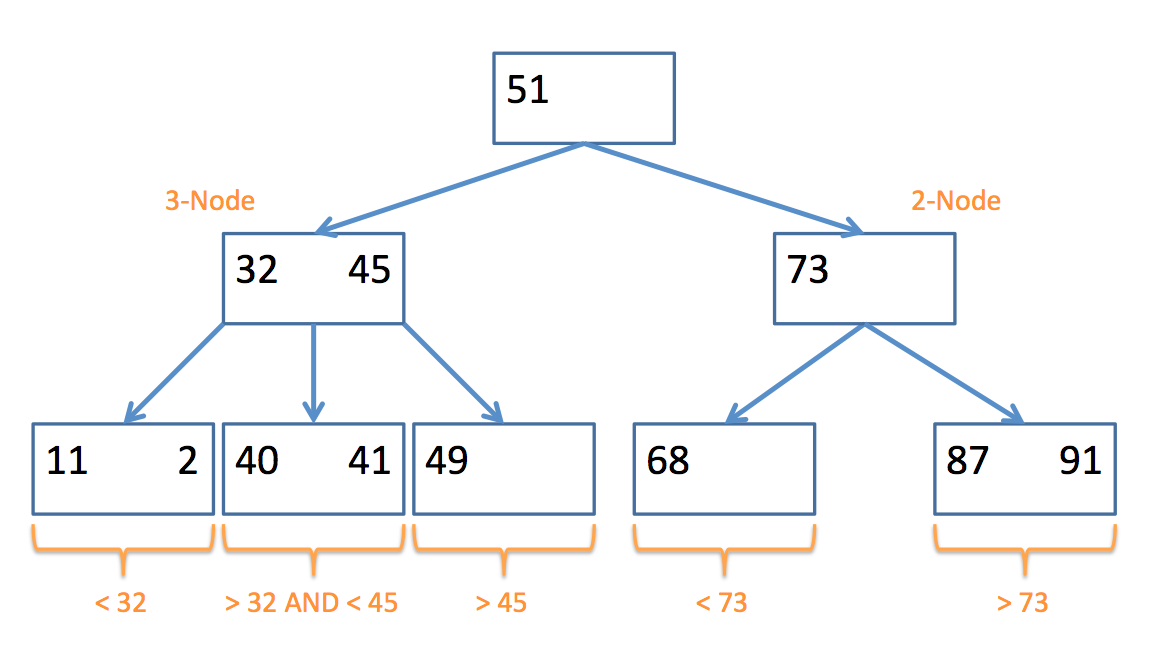
A 2-node contains 1 data element in its node, and has at most 2 children; nodes in its left subtree are less than it, and nodes in its right are greater than (or equal to) it.
A 3-node contains 2 data elements in its node (a left and a right value), and has at most 3 children; nodes in its left subtree are less than the left value, nodes in its middle subtree are between the left and the right, and nodes in its right subtree are greater than (or equal to) the right value.
Here's an example of a 2-3 Tree and the types of nodes they contain:
Insertion
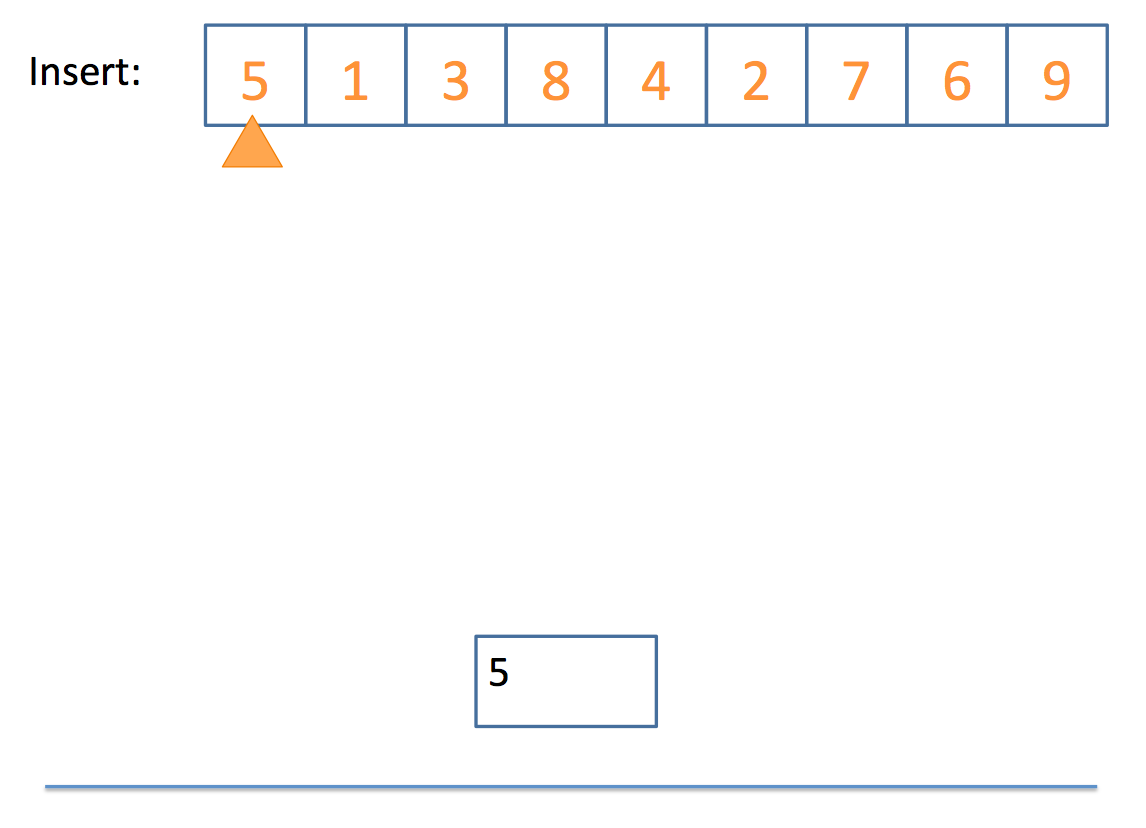
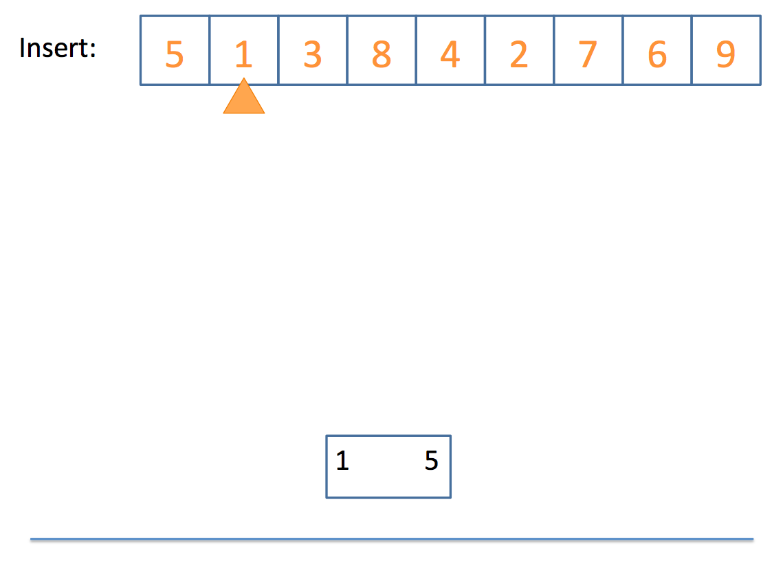
So how do we actually end up with a 2-3 tree? Well, the algorithm can be boiled down to the following pseudocode:
  // insert algorithm:

  if the tree is empty, insert a 2-Node with the value
  else, traverse the tree to find where the value goes
      once you find the node
          if that node is a 2-Node
              add the value to make it a 3-Node
          else
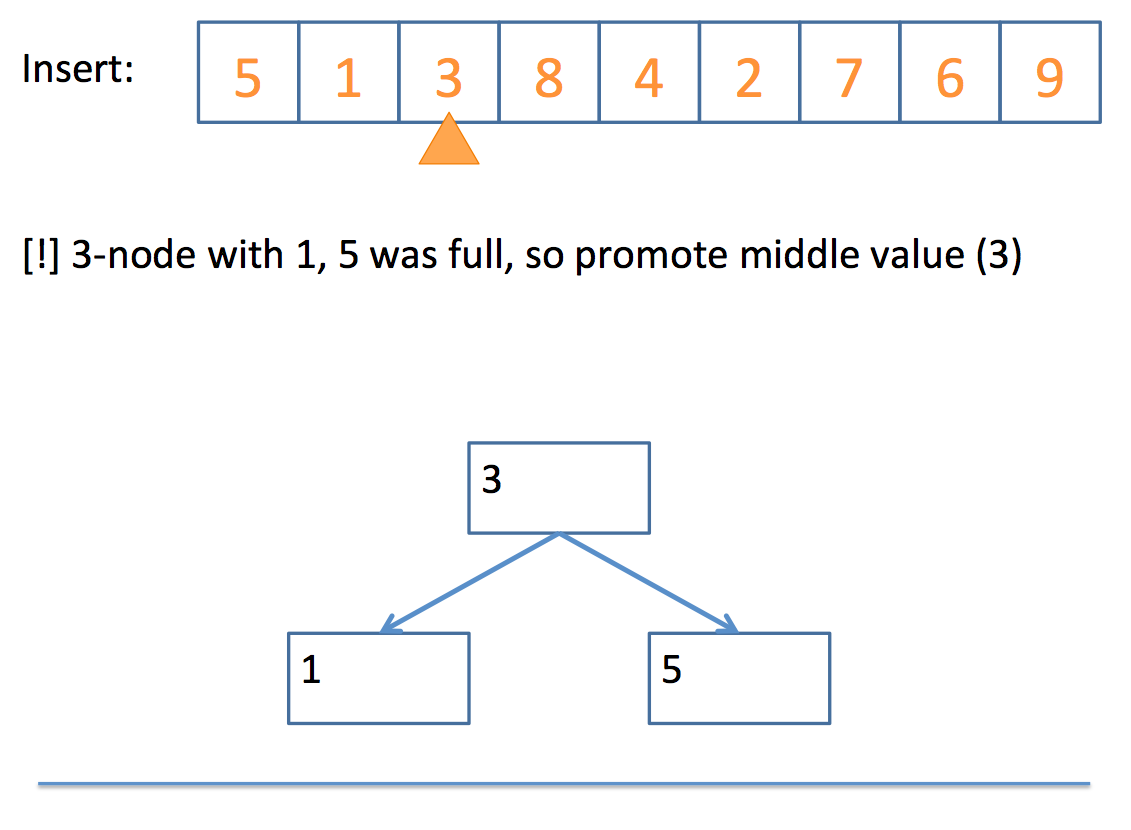
              promote the middle value to the parent


  // promote algorithm:

  if the parent is a 2-Node
      add promoted value as 2nd value, making it a 3-Node
      children placed according to relation to parent values
  if the parent is a 3-Node
      promote the middle value of those three (recursive call)
  if no parent
      promote the middle value to its own 2-Node
      split the remaining 2 values into their own 2-Nodes
      children placed according to relation to new 2-Nodes
Whew! That looks complicated, but let's look at a simple example, step by step:
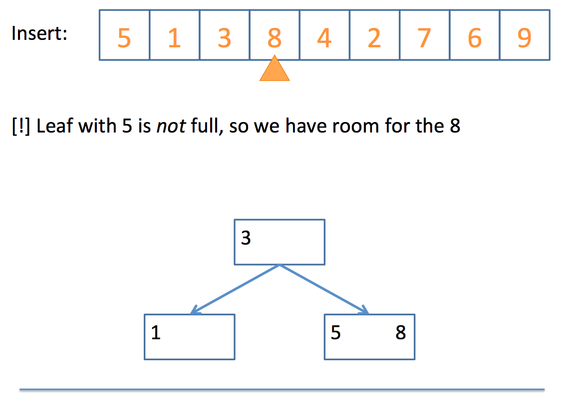
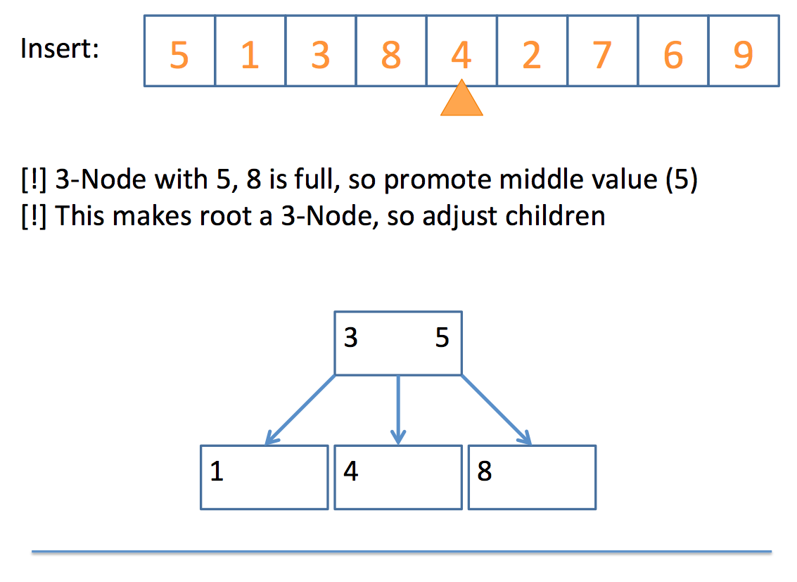
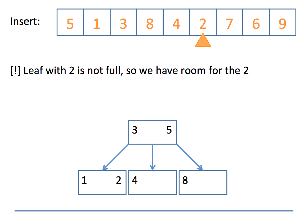
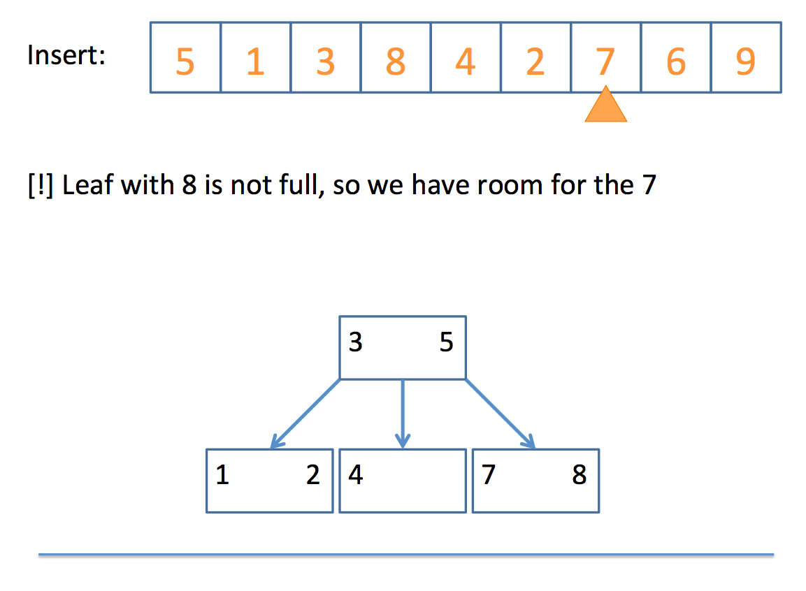
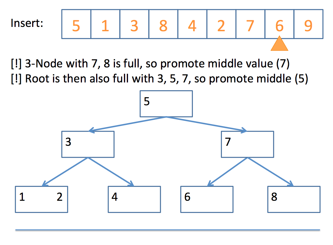
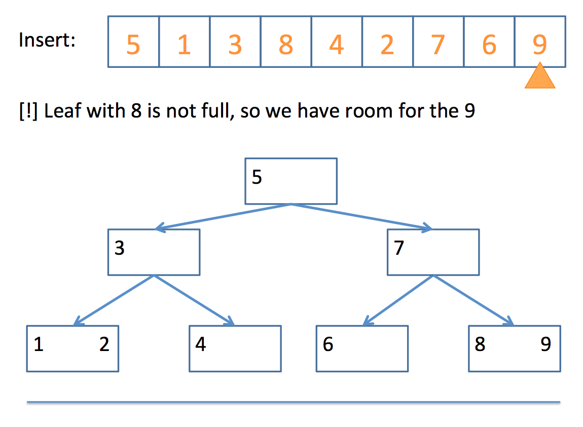
And there you have it!
Deletion is substantively more complicated and won't be detailed in this lecture.
There are many articles and videos on the topic that a simple Google search will demonstrate, but for which we simply don't have time in discussion.
STL Set & Map
Let's take a whirlwind tour through two STL collections: the set and the map
#include <set>
Sets are simply a collection of items of the given templated type stored in a binary search tree.
Here's an example of some common operations with sets:
  int main () {
      set<int> s;

      // Inserting values into set
      s.insert(5);
      s.insert(20);
      s.insert(2);

      // You can erase values from the set
      s.erase(2);
      s.insert(3);

      // You can define iterators
      // [!] This is a binary search tree,
      // what will get printed out?
      set<int>::iterator sit = s.begin();
      while (sit != s.end()) {
          cout << *sit++ << endl;
      }

      // Get the size of the set
      cout << "size: " << s.size() << endl;

      // Clear the set
      s.clear();
  }
#include <map>
Maps are simply a collection of key/value pairs (associations) of the given templated types stored in a binary search tree.
  int main () {
      map<string, int> m;

      // Inserting values into map
      m["look"] = 3;
      m["at"] = 20;
      m["me"] = 10;
      // [!] Note! Unlike vectors, in which the
      // bracket operator is undefined when the
      // index is out of range, this insertion
      // method is OK for keys that haven't been
      // set yet

      // You can erase values from the map
      m.erase("look");
      m["yo"] = 15;

      // You can update existing values
      m["me"] = 12;

      // You can define iterators
      // [!] This is a binary search tree,
      // what will get printed out?
      map<string, int>::iterator mit = m.begin();
      while (mit != m.end()) {
          // [!] Keys in iterators are stored in a
          // "first" field; values in a "second" field
          cout << mit->first << ": " << mit->second << endl;
          mit++;
      }

      // Get the size of the map
      cout << "size: " << m.size() << endl;

      // Clear the map
      m.clear();
  }
Practice & Review
Complexity Review
There were a significant number of questions regarding time complexity in the logarithmic case.
Since tree algorithms generally involve some flavor of a log complexity, let's review some algorithms now...
A rule of thumb for logarithm complexity is when you're omitting or ignoring some number of input elements with every step that is proportional to the log of the size of the input.
Often, this is manifest in divide-and-conquer algorithms, but sometimes it's simpler than that... that for example the following:
What is the time complexity of the following function?
  void someFunc (vector<int> v) {
      for (int i = 1; i < v.size(); i *= 2) {
          cout << v[i] << endl;
      }
  }
We also know that some algorithms can have logarithmic components that rely on other components of the algorithm, and vice versa...
What is the time complexity of the following function?
  void someFunc (vector<int> v) {
      for (int i = 0; i < v.size(); i++) {
          for (int j = i; j > 0; j /= 2) {
              if (v[j] == v[i]) {
                  cout << v[i] << endl;
              }
          }
      }
  }
You should also be aware that big-O complexity need not be reliant upon a single input; you can have complexities in terms of multiple inputs as well!
What is the time complexity of the following function?
  // [!] Consider N = v1.size() and M = v2.size()
  void someFunc (vector<int> v1, vector<int> v2) {
      for (int i = 0; i < v1.size(); i++) {
          for (int j = 0; j < v2.size(); j += 2) {
              if (v1[i] == v2[j]) {
                  cout << v1[i] << endl;
              }
          }
      }
  }
Lastly, let's remember our tree algorithm complexities...
What is the time complexity of the following function?
  // [!] Consider N = v1.size() and M = s.size()
  void someFunc (vector<int> v1, set<int> s) {
      for (int i = 0; i < v1.size(); i++) {
          if (s.find(v[i]) != s.end()) {
              cout << v1[i] << endl;
          }
      }
  }
Binary Tree Review
We've seen some traversal algorithms for binary trees, but let's look at a couple extra for practice.
Below, I've gotten us started with a Binary Tree class, as well as a new way to insert Nodes with a given path to an empty space.
  struct BinTree {
      // BinTreeNode struct internal
      // to the BinTree
      struct BinTreeNode {
          int data;
          BinTreeNode* left;
          BinTreeNode* right;
          BinTreeNode(int d) {
              data = d;
              left = nullptr;
              right = nullptr;
          }
      };

      // Root just points to a single
      // BinTreeNode
      BinTreeNode* root;

      BinTree() {
          root = nullptr;
      }
      ~BinTree() {}; // TODO!
      void insertAt (int i, string path);
  };
Now, suppose I wish to define the insertAt member function:
  // Creates a new node with the given data member
  // if input string p specifies a path in terms of
  // L and R children to follow to an empty spot in
  // the tree
  // The path p will look like some string of "LRL"
  void BinTree::insertAt (int data, string p) {
      BinTreeNode* b = root;
      BinTreeNode* last = nullptr;
      int i = 0;

      // First, we'll go through our desired path
      // of insertion
      while (i < p.length()) {
          // If we hit the nullptr before we're
          // done, just break out of the loop
          if (b == nullptr) {
              break;
          }
          // Keep track of our parent node...
          last = b;
          // ...then move on to the path's desired
          // child
          b = (p[i] == 'L') ? b->left : b->right;
          i++;
      }

      // If we followed a path the length of
      // our desired path, then we have a valid
      // insertion; otherwise the path was
      // mis-specified
      if (i == p.length()) {
          // If there's already a node there,
          // bad path, so we'll just return
          if (b != nullptr) {
              return;
          }
          // Otherwise, there's an opening, so
          // we'll make a new node at b
          b = new BinTreeNode(data);
          // If there's nothing in the tree yet,
          // then b is our root!
          if (root == nullptr) {
              root = b;
          }
          // If we have a parent node to add
          // the child to, update its left or
          // right pointer
          if (last != nullptr) {
              if (p[i - 1] == 'L') {
                  last->left = b;
              } else {
                  last->right = b;
              }
          }
      }
  }
So, if I wanted to add Nodes to my tree, I would simply say:
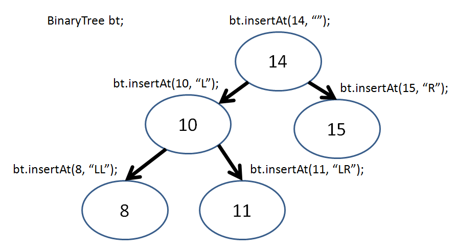
So, now I can recreate this tree in my BinaryTree class via:
  int main () {
      BinTree bt;
      bt.insertAt(14, "");
      bt.insertAt(10, "L");
      bt.insertAt(8, "LL");
      bt.insertAt(11, "LR");
      bt.insertAt(15, "R");
  }
Neat! Now let's look at making some of our own functions...
First, let's have a way to print out our tree; we'll print out each subtree as enclosed within parentheses, like so:
  int main () {
      BinTree bt;

      bt.insertAt(14, "");
      // prints: (14)
      printByClosure(bt.root);
      cout << endl;

      bt.insertAt(10, "L");
      // prints: ((10)14)
      printByClosure(bt.root);
      cout << endl;

      bt.insertAt(8, "LL");
      // prints: (((8)10)14)
      printByClosure(bt.root);
      cout << endl;

      bt.insertAt(11, "LR");
      // prints: (((8)10(11))14)
      printByClosure(bt.root);
      cout << endl;

      bt.insertAt(15, "R");
      // prints: (((8)10(11))14(15))
      printByClosure(bt.root);
      cout << endl;
  }
Complete the function shell for printByClosure below:
  void printByClosure (BinTree::BinTreeNode* b) {
      // [!] Base case
      if ( ??? ) {
          ???
      }

      // [!] Otherwise, starting a new
      // closure, so print out...
      cout << ???;

      // [!] Perform some form of traversal
      // here... which one will give us the
      // desired output?

      // [!] Ending our closure, so print...
      cout << ???;
  }
Let's do something "fun"... why don't we create a function that turns our tree into a mirror image of itself?
  int main () {
      BinTree bt;
      bt.insertAt(14, "");
      bt.insertAt(10, "L");
      bt.insertAt(18, "R");
      printByClosure(bt.root);
      cout << endl;
      // Was ((10)14(18)),
      // Now ((18)14(10))
      mirror(bt.root);
      printByClosure(bt.root);
      cout << endl;

      bt.insertAt(17, "LR");
      printByClosure(bt.root);
      cout << endl;
      // Was ((18(17))14(10)),
      // Now ((10)14((17)18))
      mirror(bt.root);
      printByClosure(bt.root);
      cout << endl;
  }
Complete the function shell for mirror, below:
  void mirror (BinTree::BinTreeNode* b) {
      // [!] Base Case
      if ( ??? ) {
          return;
      }

    // Create a temp holder for our swap
      BinTree::BinTreeNode* temp;

    // [!] Perform some order of traversal
    // to do the swap... which one?
      ???

    // [!] Swap the current node's left
    // and right with the temp, saving
    // one into temp first
      ???
  }
  // ^ Example credit to Stanford's tree examples
  // (listed later)
I'll have some more examples using this class on the practice final...