Questions from Last Week
Q: Is there a particular "magic load factor" that guarantees Hash Table constant time performance on its operations?
A: Well, I don't know about "magic," but as it turns out, many implementations aim for a load factor < 0.7 lest too many collisions start to happen.
Q: Is it possible to get a "perfect" hash function to avoid any collisions?
A: Yes, but only when you know all of your keys in advance. Such "perfect" hashes are useful when you have frequent look-ups of a large hash table with infrequent (or no) updates.
You can read more about perfect hashes on the Wiki article.
Heaps
Let's talk about a new tree data structure. The heap!
WARNING: The heap data structure is on no way related to the heap where dynamically allocated variables are stored!
Such unfortunate naming schemas in computer science... it's not like humans have infinite generative language capacities or anything...
To break the ice, here's another topical XKCD because you guys seem to love these as much as I do:
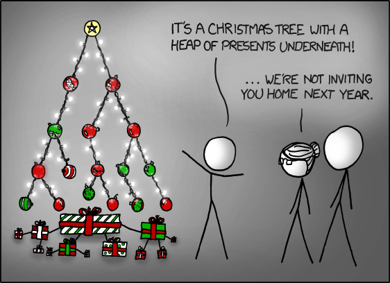
A heap (generally referring to a max heap) is a special type of tree where *all* subtrees of a given Node have values less than or equal to that Node's.
In the above comic, we see that the heap of presents at the base has the largest at the top with children decreasing in size with greater depth.
Our discussion, however, will be restricted to binary heaps, which have some additional restrictions.
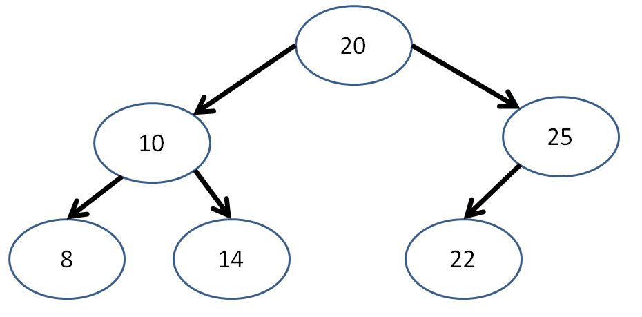
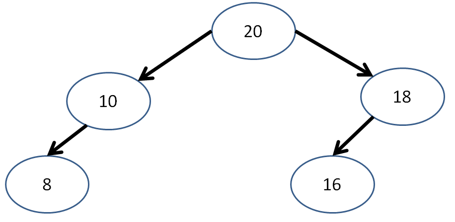
A binary heap is a complete binary tree where all subtrees of a given Node have values less than or equal to that Node's.
So we're restricting the number of children any Node can have to 2, AND requiring the binary tree be complete.
A complete binary tree is a binary tree with all full levels, except for possibly the last level, in which case it is required that the Nodes be filled from left to right without any spaces.
Is the following binary tree complete? Is it a heap?
Is the following binary tree complete? Is it a heap?
Is the following binary tree complete? Is it a heap?
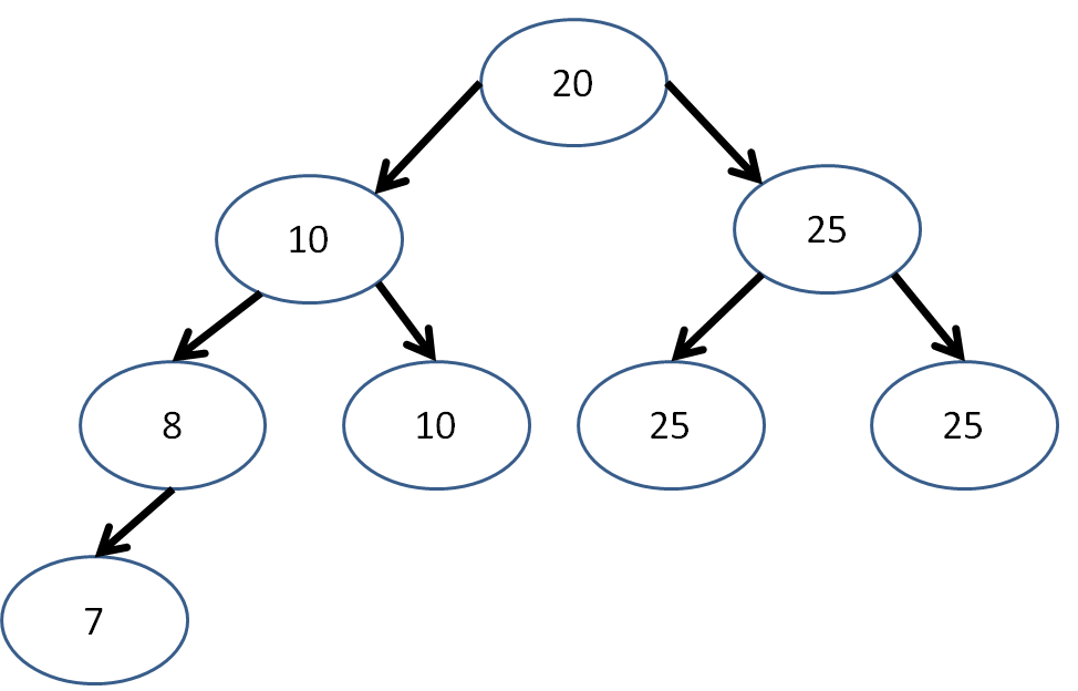
Is the following binary tree complete? Is it a heap?
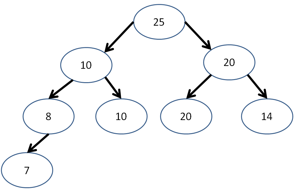
Is a single-node tree a heap?
Yes! It must be complete because the last (and only) level is full, and its value must be larger than its subtrees because it has no subtrees!
How many unique structural configurations (ignoring node values) are there for a complete binary tree with N nodes?
Just 1! If you were to change the position of any node in the structure, it would cease to be complete.
Heap Properties
Heaps have some nice properties, for example:
The largest value of a (max)heap is always at the root, and therefore accessible with constant time!
Because heaps are complete trees, we can represent them as arrays to enable random access, with indexing starting at the root and numbering nodes level-by-level from left-to-right.
What performance benefit does representing a complete tree as an array have over a Node-with-pointers implementation?
Arrays are indexed, meaning we can access any element with constant time.
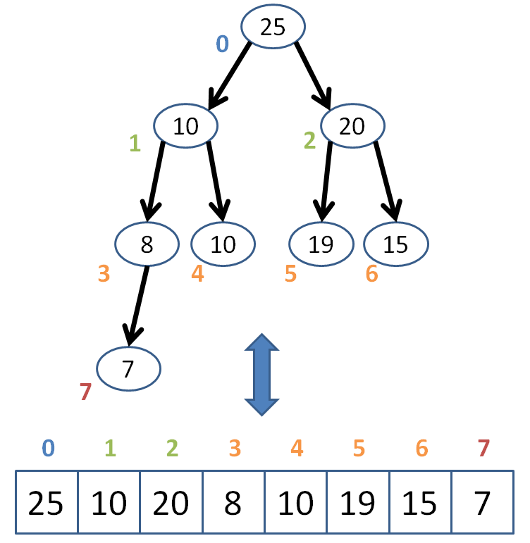
"Nice colors in that graph, Andrew, do you also design children's play equipment?"
Shhh! It was illustrative!
We know that in the array representation of a heap, the root must always be at index 0.
But how do we determine the children and parent of any given index in an array?
Well, since it's a complete tree, we have a simple computational way of finding these indexes...
Given the index n of a "Node" in our conceptual tree structure, how can I get the index of the parent?
Index of parent: (n - 1) / 2; (NOTE: this is integer division, so we ignore the decimal of the quotient)
So, we can define a simple functional mapping:
  int getParent (int index) {
      return (index - 1) / 2;
  }
Getting the left and right children is a similar mechanical exercise:
  // Child is either 'L' or 'R'
  int getChild (int index, char child) {
      int result = (index * 2) + 1;
      if (child == 'R') {
          result++;
      }
      return result;
  }
Draw the binary tree representation of the following heap:
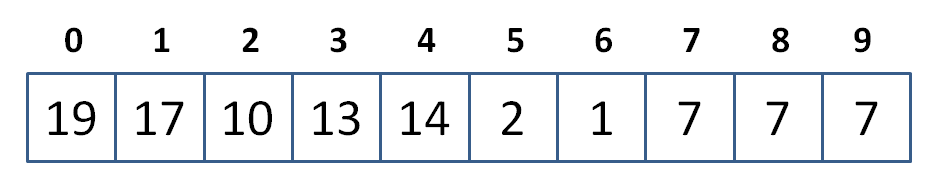
Now that we have the basic tools down, we're ready to go over some heap algorithms!
Heap Operations
Insertion
After every operation on a heap, we have some general steps: perform the operation and then "reheapify" the binary tree.
For insertion, that looks like this:
Create a complete binary tree with the newly inserted node in its proper location as the right-most vacant leaf position on the last level of the tree.
Starting at that newly inserted node, bubble upwards ensuring that each node is less than its parent.
As soon as a parent is greater than the node we're bubbling, stop--your array is now reheapified! (assuming it was a heap before the insertion).
Why is it sufficient to conclude that in step 3, when the parent is greater than the node we're bubbling, that we may stop? Why must we not also continue checking farther up the heap to verify its heapiness?
By assumption, we are inserting into a structure that is already a heap. This means that all nodes are already abiding by the definition of a heap. So, when we insert a new node, and stop bubbling up whenever the parent is larger than what we're bubbling, we can trust that all nodes updwards are already heap-compliant.
Using the above steps, insert the node with value 50 into the heap below:
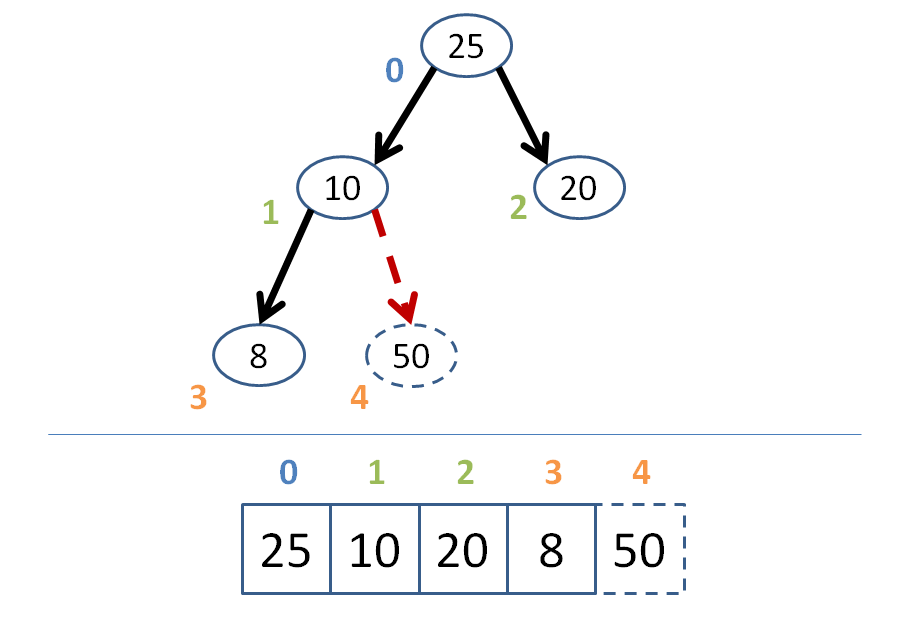
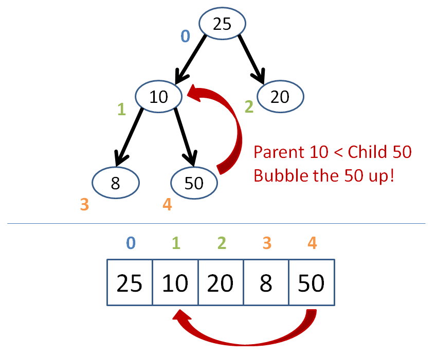
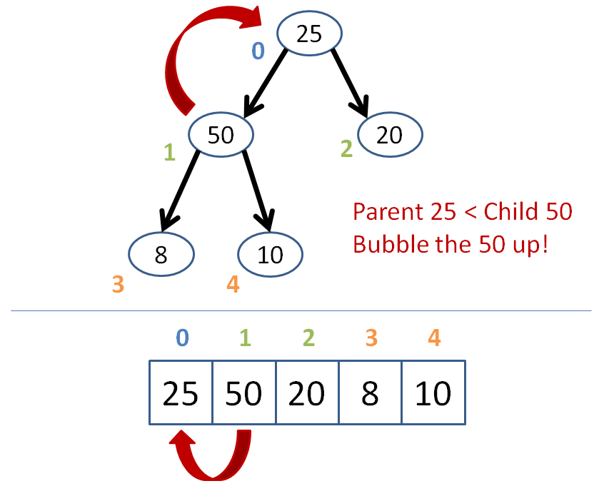
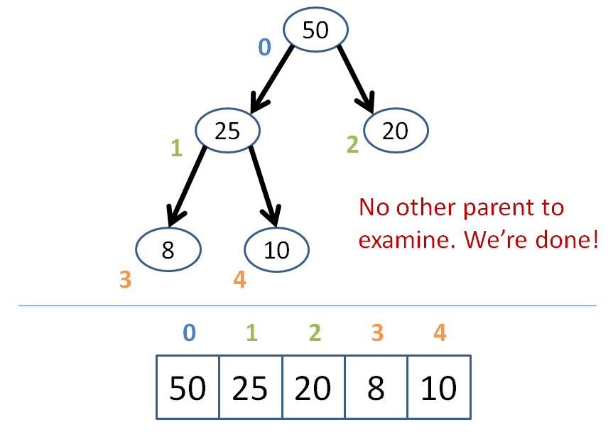
Got that?
Let's make a simple BinaryHeap class with this algorithm!
I'll start you off...
Complete the insert function and its helper, bubbleUp, in our BinaryHeap below:
  template <typename T>
  class BinaryHeap {
      private:
          vector<T> heap;

          // Traversal helpers
          int getParent (int index) {
              return (index - 1) / 2;
          }
          int getChild (int index, char child) {
              int result = (index * 2) + 1;
              if (child == 'R') {
                  result++;
              }
              return result;
          }

          // Continues to bubble values up the
          // tree until we find a node that is
          // greater than it
          void bubbleUp (int index) {
              // [!] If we're at the root, then
              // we're done
              if ( ??? ) {return;}

              // [!] Get parent index and store it
              int parent = ???;

              // [!] If the parent's value is less than
              // the current one's...
              if ( ??? ) {
                  // [!] ...then we swap them...
                  ???

                  // [!] ...and recurse on the new parent!
                  bubbleUp(parent);
              }

          }

      public:
          void print () {
              for (int i = 0; i < heap.size(); i++) {
                  cout << heap[i] << endl;
              }
          }

          void insert (T toInsert) {
              // [!] Add new element to next available
              // slot in the binary tree
              ???

              // [!] Start bubbling values up from
              // the newly added value
              ???
          }
  };
Now let's test it using our example from before!
  int main () {
      BinaryHeap<int> b;
      b.insert(25);
      b.insert(10);
      b.insert(20);
      b.insert(8);

      cout << "BEFORE adding 50:" << endl;
      b.print();

      b.insert(50);
      cout << "AFTER adding 50:" << endl;
      b.print();
  }
Great! On to deletion.
Deletion
Nothing particularly surprising about deletion; it's essentially the same algorithm as insertion, in reverse!
Remove the target node from the heap
Promote the bottom-right-most leaf of the last level to the position of the removed node
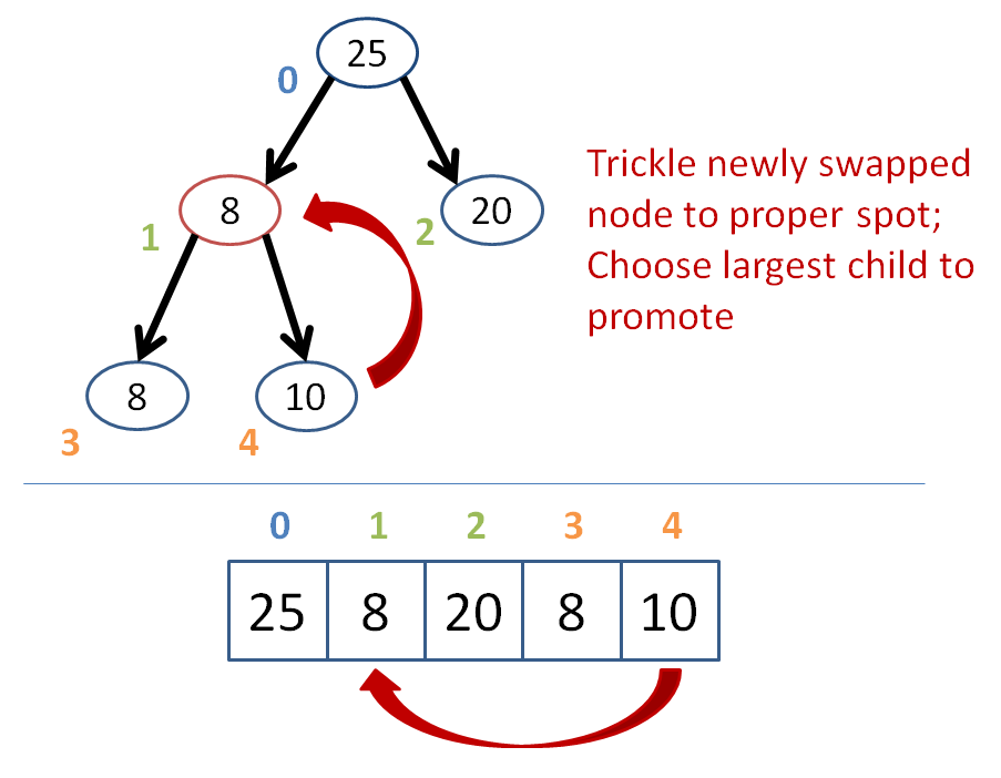
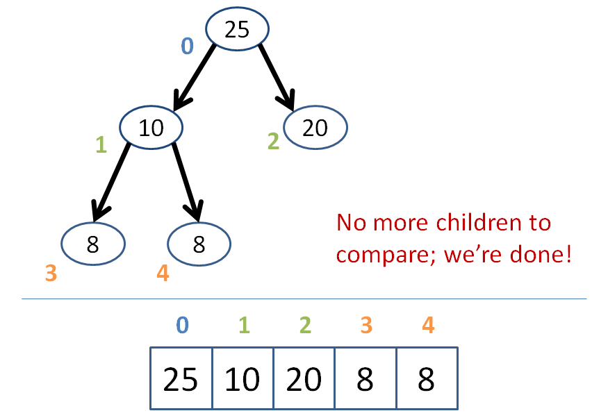
Trickle down the promoted item such that if either of its two children are greater than it, then it trades places with the greatest of its children.
Continue trickling down until no child is greater than the trickling node.
Let's try removing the 50 node at the root from the heap below:
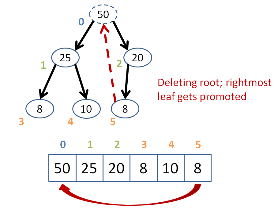

I shall leave it as an exercise to implement the deletion function into our BinaryHeap class!
What is the time complexity of insertion? Of deletion?
Both are O(log(n)), for the same reason that binary search was. At each step of bubbling, we're ignoring 1/2 of the other nodes in the heap.
To find an element in a heap, can we perform the same binary search algorithm on heaps that we can on binary search trees?
No, we do not have the same guarantee that an item must be found in one subtree or another; it could be at either if it is less than a given Node N.
Heap Applications
Heaps are nice for a variety of applications; we'll discuss a few right now!
Priority Queues
Priority queues are a data structure that use heaps for container with the restriction that removing elements from the heap can only be done at the root.
Because we know the root of a maxheap is always the greatest element in that heap, we say that we're always removing the item with the highest priority before we get to the others.
Is the standard queue data structure that we know a special case of a priority queue? What property of items in a standard queue would cause them to behave like a priority queue?
Yes! Standard queue items are simply removed in the FIFO order of their insertion; we could mimic this behavior with a priority queue by simply time stamping the time of insertion and always removing the one with the earliest time stamp first.
Huffman Coding
Suppose I wish to transmit a text message using the least amount of data as possible.
Since text is composed of characters, most general-purpose encoding schemas (like ASCII) will assign some binary representation to each character, giving it a unique code that can be translated into text.
  // ASCII Bit-code Representation:
  'A' = 65 (base 10 - decimal)
      = 01000001 (base 2 - 8bit binary)

  // Character Strings:
  "AAA" = 01000001 01000001 01000001 (24 bits)
BUT, what if I don't have 256 different characters that I need to represent in my text message? How will ASCII be wasteful?
Suppose my message consists of strings of only 4 characters. ASCII would use 8 bits to represent each character, even though I only need 2 bits to uniquely represent them!
Suppose I'm using 2 bits to represent the letters {A, B, C}. I conclude that I can have bit codes translate as follows:
  // Custom Bit-code Representation:
  1  = A
  00 = B
  01 = C

  // Character Strings:
  "A"   = 1
  "BA"  = 001
  "CAB" = 01100
Suppose I then discover that the letter 'A' appears very infrequently in my text messages, and C appears very frequently. If I want to keep my bit-string representations of my text messages as small as possible, what change should I make to the above translation?
Make 1 = C and 01 = A, since the frequent appearances of C and infrequent appearances of A will result in smaller bit-strings on average.
So, it'd be nice if, for any arbitrary alphabet I wish to define (or a restricted alphabet where I know I'm only using some N number of characters), I could minimize the bit-string representation of any character-string to be parsimonious!
Huffman Coding provides an algorithm to create a binary tree that can encode and decode any string defined on an alphabet that is weighted by its character frequency.
That too is a lot of words... what it means is that we have a way to generate bit string encoding schemas that minimize the number of bits we'd need to use to express a character-string in our alphabet (on average).
Let's see how it works!
Encoding
Produce a Huffman Encoding for an alphabet defined over 5 letters, {A, B, C, D, E} with the following frequencies:
  // Character: Frequency%
  A: 20%
  B: 30%
  C: 10%
  D: 15%
  E: 25%
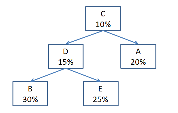
Step One: Place all of the characters into a MINHEAP priority queue, where the root will have the least frequency, and all subtrees of Node N have frequencies greater than N. In other words, nodes with the lowest frequency have the highest priority.
What will the minheap look like for the above characters, assuming I insert them in the order listed?
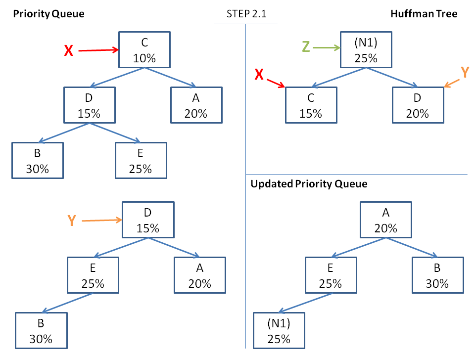
Step Two: Begin forming the Huffman Encoding binary tree. Until you are left with a single Node in the priority queue, do the following:
  Let Node X = pri_q.pop()
  // [!] Node Y created after popping to get
  // Node X, and then reheapifying
  Let Node Y = pri_q.pop()
  Create Node Z = new parent of X and Y
  Set frequency of Z = freq(X) + freq(Y)
  Insert Z into pri_q
In short, we pop the 2 least frequency-nodes in the priority queue, join them with a new parent whose frequency is the sum of those two nodes, and then add that new parent into the priority queue.
We do this until we are left with a single node, which is the root of our Huffman tree.
For our example, this will look like the following:
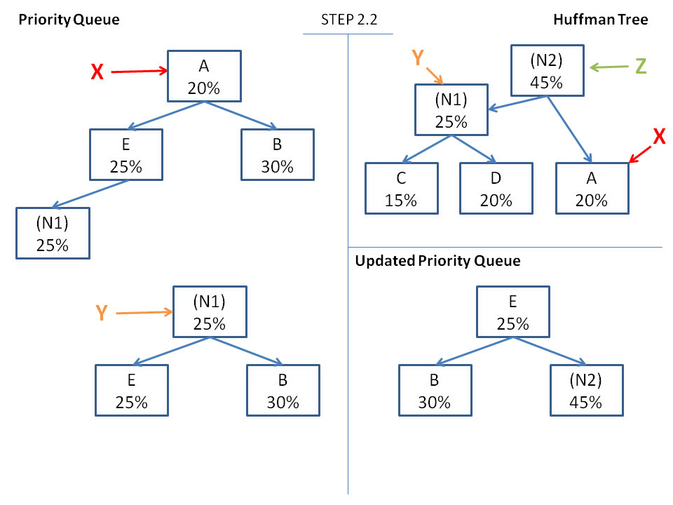
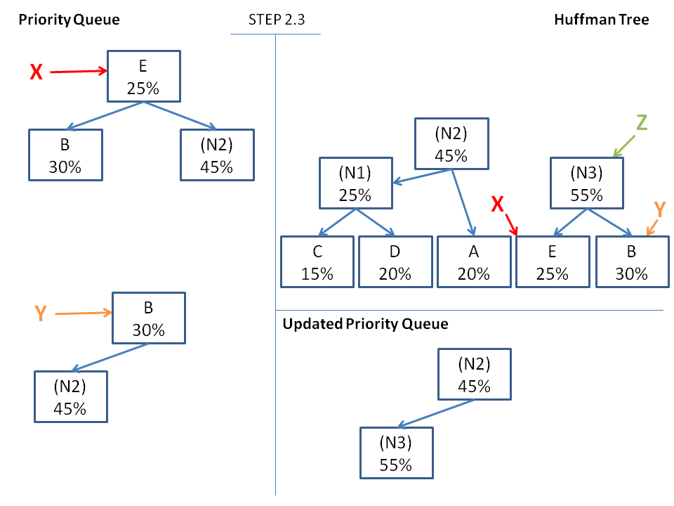
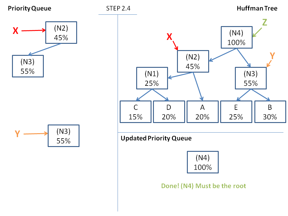
Step 3: To get an encoding for our tree, simply treat every Node's left pointer as a 0 bit and every Node's right pointer as a 1 bit, and collect bits along the path to find that character's bit code.
So, for our example, this will look like:
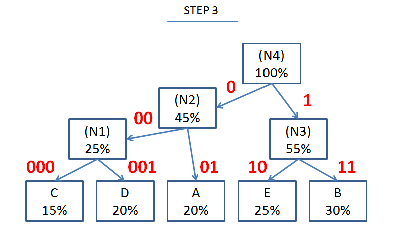
So, for example, the bit code for B = 11 and the bit code for D = 001.
Note: the most frequently used characters have the smallest bitcode! This is exactly what we wanted.
Decoding
Suppose now I have a Huffman tree, and wish to decode a message. The process for this is simple.
To decode a bit-string using a Huffman tree, start at the tree's root, follow left branches when you see a 0, or right when you see a 1, return a character whenever you reach a leaf, and then restart at the root for the next character.
Using the Huffman tree we created above, decode Andrew's old-school diss corresponding to bit-string: 00001001. (Click for solution)
CAD
So that's Huffman coding! ...you cad!
How about some conceptual questions?
Why do we use a priority queue to store the characters with their frequencies? Wouldn't it be easier to simply maintain a sorted vector?
No! Remember that we frequently insert the new parent nodes (Z) that are created in the algorithm, which would cause performance issues for vectors. Furthermore, priority queues always have the next item we need to add to the Huffman tree at the root, and are accessible with O(1), then only + O(log(n)) to reheapify, rather than O(n) to reorganize a vector. Finally, nodes popped from the priority queue can be the same nodes used in the Huffman tree, meaning we don't need to allocate anything other than the Nodes once, rather than allocating a vector AND THEN every Node in the Huffman tree, which can be expensive.
What is the computational complexity of Huffman encoding?
O(n log (n)). Popping, reheapifying, and inserting elements into the heap takes O(log(n)), and is done n times, one for each character.
Heap Sort
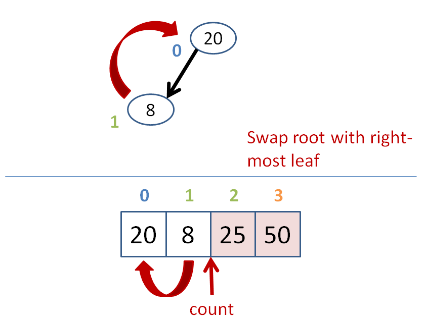
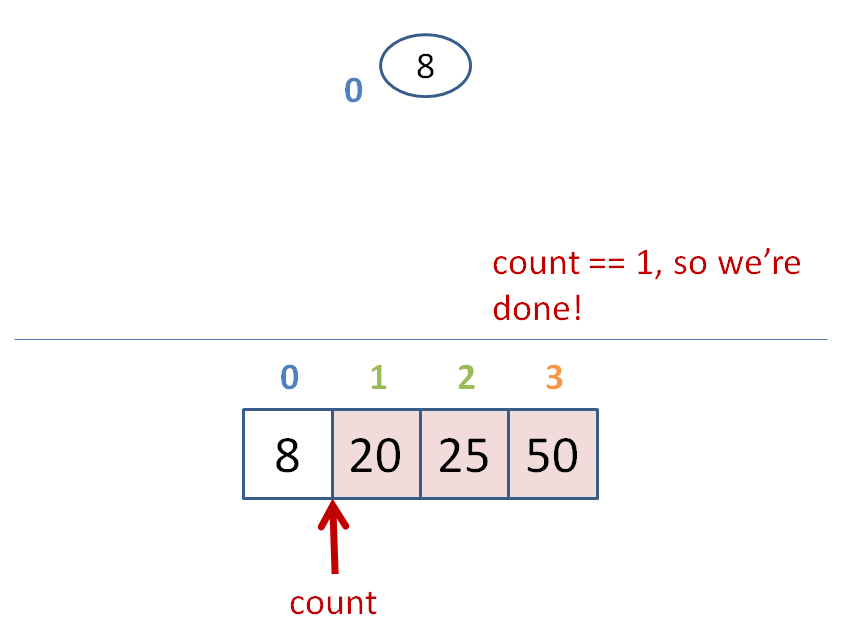
Heap sort is a way to retrieve a sorted list of a heap's elements.
Its algorithm goes something like this:
  count = size of heap
  while count > 1
      heapify the heap
      swap the root with the deepest, right-most leaf
      count--
Since we are representing heaps in their array format, what we are left with after heapsort is a sorted array of that heap's elements.
Let's do some heap sorting!
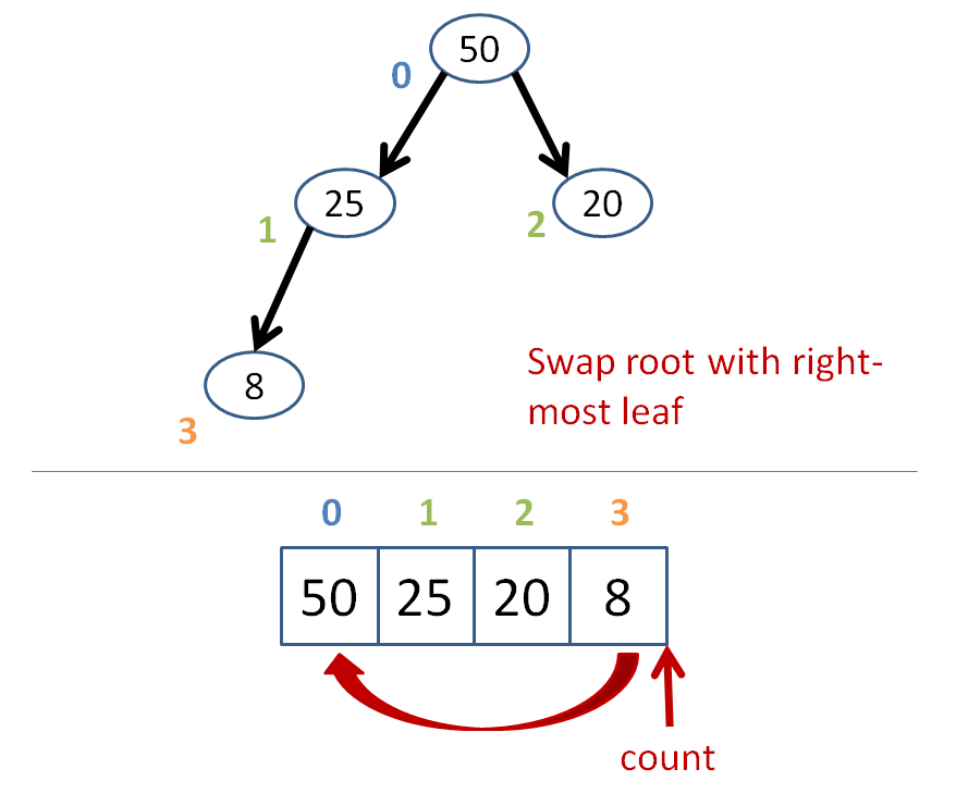
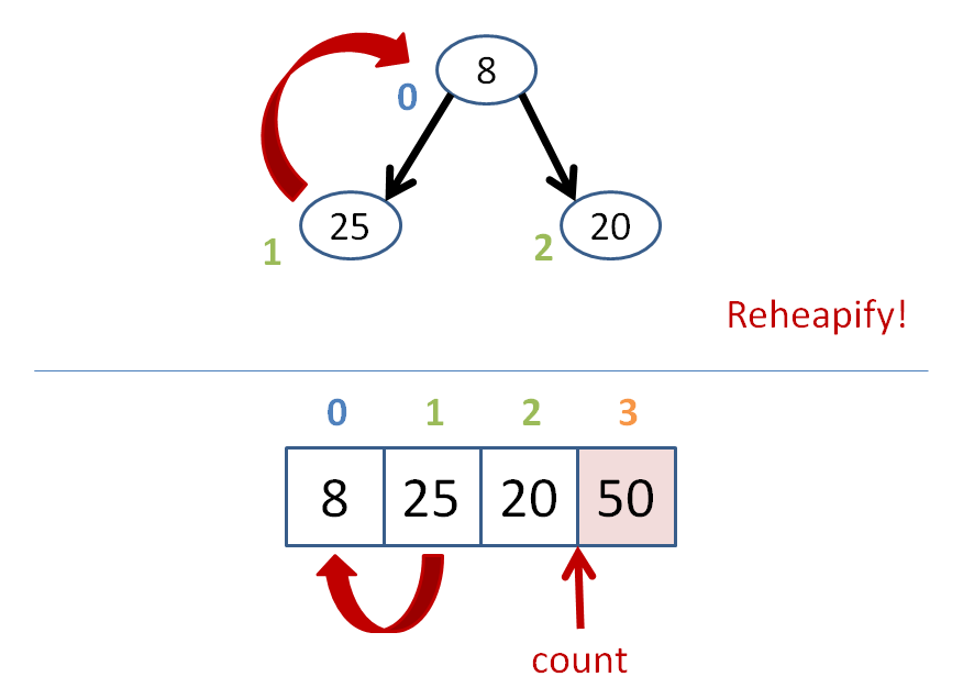
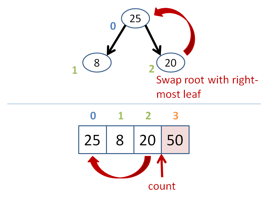
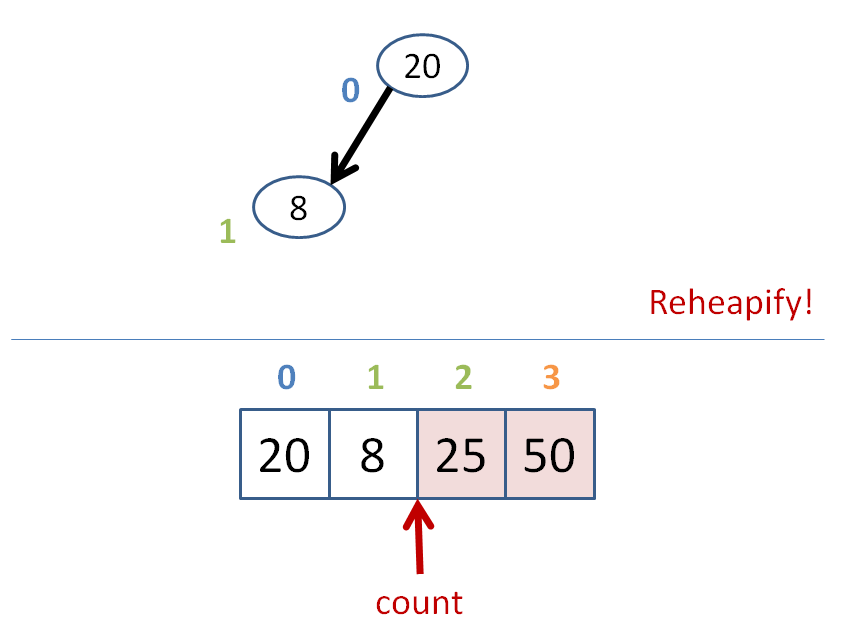
What is the time complexity of heapsort?
Heap sort has time complexity O(n*log(n)), like most other gold standard sorts, since "heapifying" takes log(n) time, and is done n times, for each element.
Heapsort takes less space than merge sort, but isn't possible to perform in parallel, unlike merge sort.
Graphs
Graphs are about as fun as a data structure can get (if you ask me).
A graph is an abstract data type consisting of some number of Nodes connected by some number of edges, which may be directed or not.
Such a loose definition! Let's look at a graph...
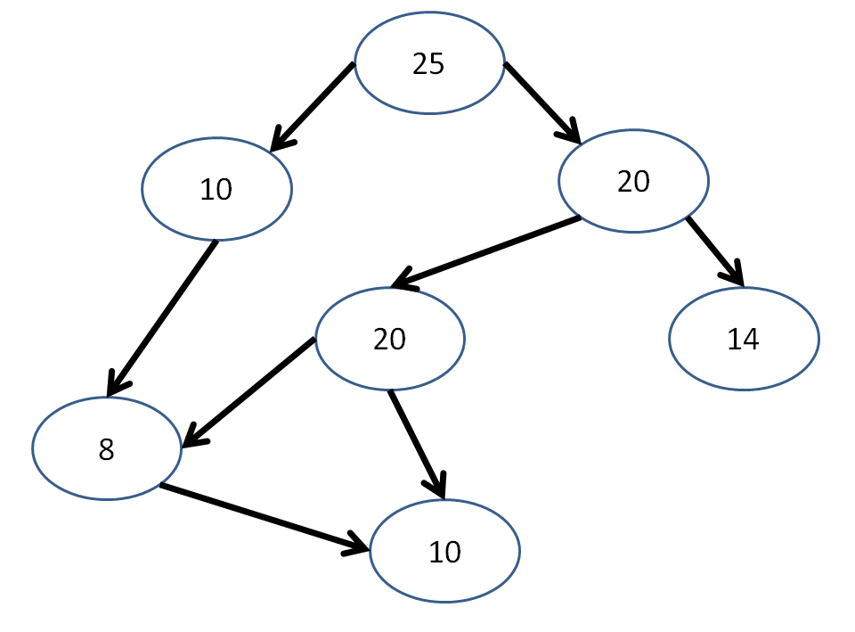
Seeing how a graph is just any collection of nodes and edges, let's think for a second...
Are all trees also graphs?
Yes! Trees are just graphs with some additional constraints (which we'll see in a moment).
Are all graphs also trees?
No! Graphs can have a variety of properties that violate the constraints of trees; let's see those in the following table.
Property |
Trees |
Graphs |
|---|---|---|
Notion of root |
Yes |
Not necessarily |
One path from root to any node |
Yes |
Not necessarily |
Can contain cycles |
No |
Yes |
Nodes can have multiple inbound arrows |
No |
Yes |
Have methods of traversing nodes |
Yes |
Yes* |
I put a star next to the graph capacity for traversal simply because, unlike with, say, a binary tree, in which we have defined traversal methods like left-to-right postorder, graphs can be traversed starting at any node and following a variety of different traversal schemas.
Additionally, we're not guaranteed that we could traverse all elements of a graph, even if we have a systematic algorithm for doing so. Take the following graph, for example:
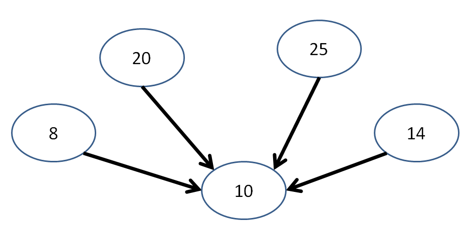
Starting at any one of these nodes, we're not guaranteed that we'll visit every other node in the graph! (in fact, in this case it's not possible)
Long story short, there are a variety of niceties we had with trees that are lost with the loose constraints of graphs... but we also gain some cool stuff too.
Graph Properties
A graph is said to be directed if every edge has at least one directed arrowhead.
This might even mean bidirected arrows with arrows on either end!
A graph is said to be acyclic if it contains no cycles.
A cycle exists in a graph whenever it is possible, by simply following some path of directed edges, to visit a node twice.
A very common graph representation involves the case where both of these properties are combined:
A directed, acyclic graph (also known as a DAG) is a directed graph with no directed cycles.
Is the following graph a DAG?
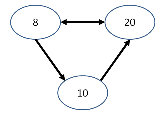
Is the following graph a DAG?
Graph Algorithms
There are a variety of graph algorithms for different applications, but for our introduction, let's just examine 1 or 2:
A depth-first traversal of a graph, starting at some node N, will visit descendants of N along a straight line of child-succession until (a) we visit a child we've already visited, or (b) we reach a leaf, at which point we backtrack to the nearest previously-visited ancestor with more children to visit.
We can use a stack to exhibit a depth-first traversal of a graph in the following manner:
  // Pseudocode
  S = Stack of vertices
  S.push(root) // pushing a vertex onto S also marks it as "visited"
  while S is not empty:
      current = S.pop() // assume popping returns vertex at front
      visit current
      for each unvisited child c of current:
          S.push(c)
A depth first traversal that remembers the nodes that it's already visited will not repeat them.
Depth first traversals are not necessarily unique!
Show a couple of depth-first traversals starting with node 1 in the following DAG:
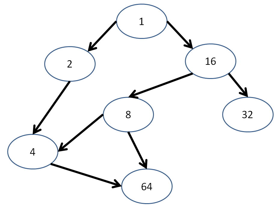
Some viable depth-first traversal:
1, 16, 32, 8, 64, 4, 2
1, 2, 4, 64, 16, 8, 32
The following are NOT viable depth-first traversals starting at node 1. Why?
1, 2, 16, 4, 8, 32, 64
1, 2, 4, 8, 64, 16, 32
A breadth-first traversal provides an ordering of nodes such that no node appears in the sequence before any of its parents. In other words, starting at Node N in the graph, a breadth-first traversal will then visit all children of N before visiting any grandchildren of N.
We can use a queue to exhibit a breadth-first traversal of a graph in the following manner:
  // Pseudocode
  Q = Queue of vertices
  Q.push(root) // pushing a vertex into Q also marks it as "visited"
  while Q is not empty:
      current = Q.pop() // assume popping returns vertex at front
      visit current
      for each unvisited child c of current:
          Q.push(c)
This is useful for tracing dependencies where we have to resolve the parents before the children!
What are some viable breadth-first traversals of the following graph?
A viable breadth-first traversal: 1, 2, 16, 4, 8, 32, 64
Representing Graphs
OK cool, but how do we store these graphs? What data structures can we use to represent them?
An adjacency matrix is a 2D array with a row / column for every node, and an indication at index [i][j] of whether node i is connected to node j.
Usually we indicate adjacencies with the number 1 to represent an edge going from node i to node j, and a 0 if there is no edge between them.
For example, an adjacency matrix denoting the graph (where each matrix index i corresponds to the node with value 2^i; so, for example, [0][1] corresponds to the edge from the node with value 1 to the node with value 2) above might look like:
       1  2  4  8  16 32 64
  1   [0, 1, 0, 1, 0, 0, 0]
  2   [0, 0, 1, 0, 0, 0, 0]
  4   [0, 0, 0, 0, 0, 0, 1]
  8   [0, 0, 1, 0, 0, 0, 1]
  16  [0, 0, 0, 1, 0, 1, 0]
  32  [0, 0, 0, 0, 0, 0, 0]
  64  [0, 0, 0, 0, 0, 0, 0]
Problem: this matrix can have a lot of 0s and waste space when there aren't many edges in our graph.
An adjacency list stores each edge connection as a vector of lists of ints, where each index contains the ints representing the nodes
For example, an adjacency list for the above graph might look like (ignoring the index-to-node-value gymnastics we did above with the adjacency matrix):
  1  [] -> 2 -> 16
  2  [] -> 4
  4  [] -> 64
  8  [] -> 4 -> 64
  16 [] -> 8 -> 32
  32 []
  64 []
Problem: this adjacency list can be wasteful when our graph has a lot of edges.
We are best off using adjacency matrices when we have a lot of edges between nodes, but not a lot of nodes... and best off using adjacency lists when we have a lot of nodes but not a lot of edges.
Graph Applications
Graphs are very often used to represent geographical data and distances between points.
For this reason, one of the most ubiquitous graph algorithms helps us compute efficient distances between nodes in a graph.
Given a graph with nodes = geographical locations, and edges connecting adjacent locations with some distances between them, Djikstra's algorithm tells us the least distance we would have to travel from a given node S to any other node in the graph.
The following example graph lists locations A through E that are separated by distances indicated along the edges.
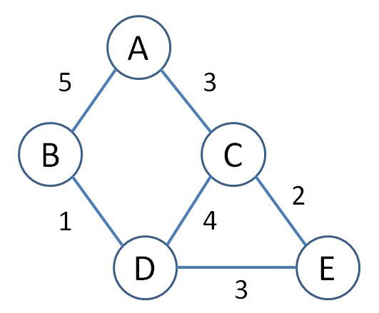
What is the shorted distance from A to E? What path does it take?
A -> C -> E, with a total cost of 5.
So, we'd like to have a way of automatically computing the shortest distance from a node to every other node in the network. Enter Djikstra's algorithm!
Djikstra's algorithm operates by maintaining two vectors:
dist: for each node, tracks the optimal distance from the start node. Each element in this vector starts out with value infinity, except for the start node, which starts out with value 0.
done: for each node, tracks whether or not we have already computed the optimal travel distance from it to its neighbors. Each element in this vector starts out as false, except for the start node, which starts out as true.
  function Djikstra(graph, start):
      initialize dist, done (as stated above)
      set node u = start
      while done still has 1 element false:
          u = min distance, not done node from start
          done[u] = true
          for each node v in unvisited neighbors(u)
              d = distance(u, v)
              if d + distance(s, u) < dist[v]
                  dist[v] = distance(s, u) + d
Let's trace this algorithm through our example now.
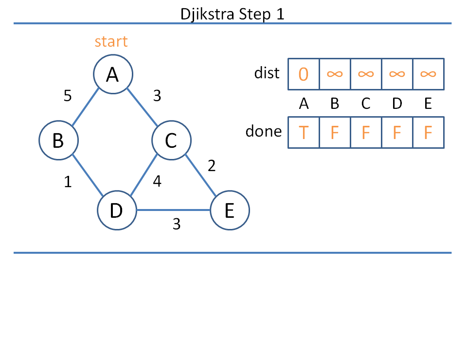
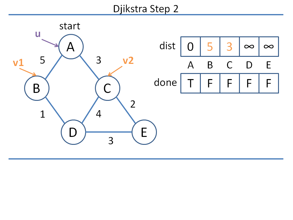
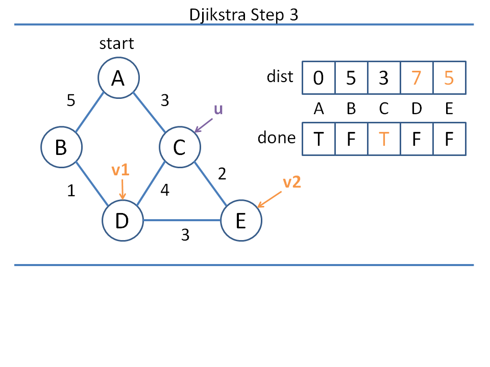
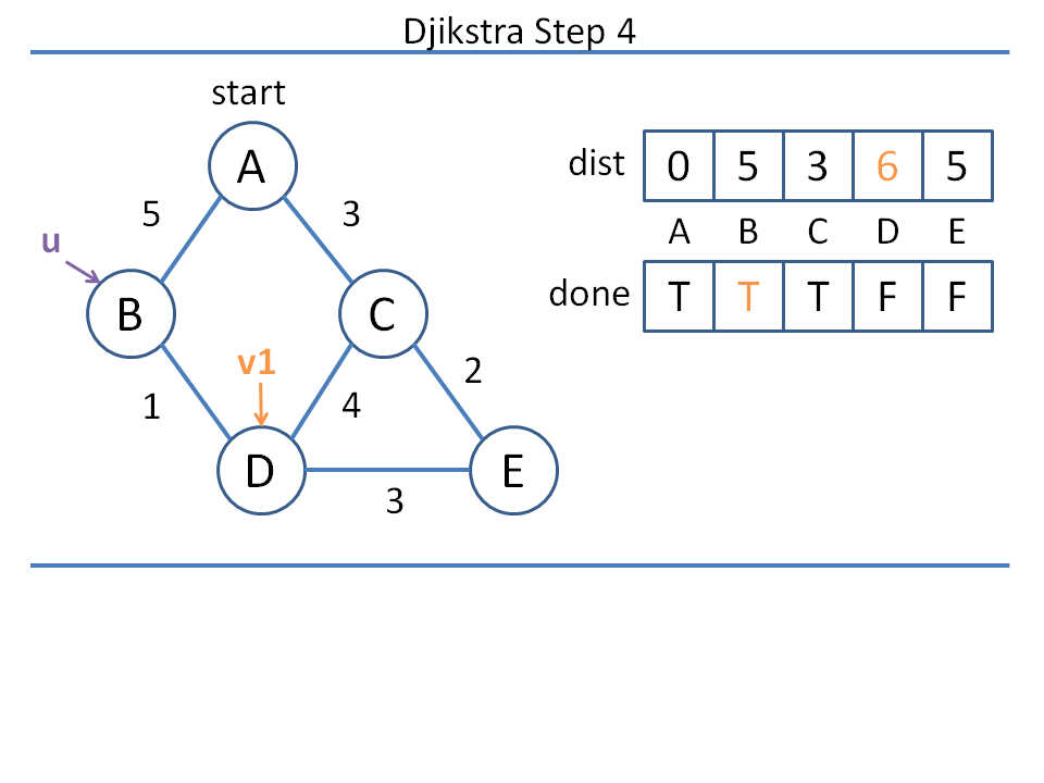
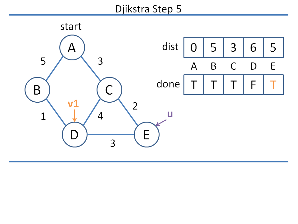
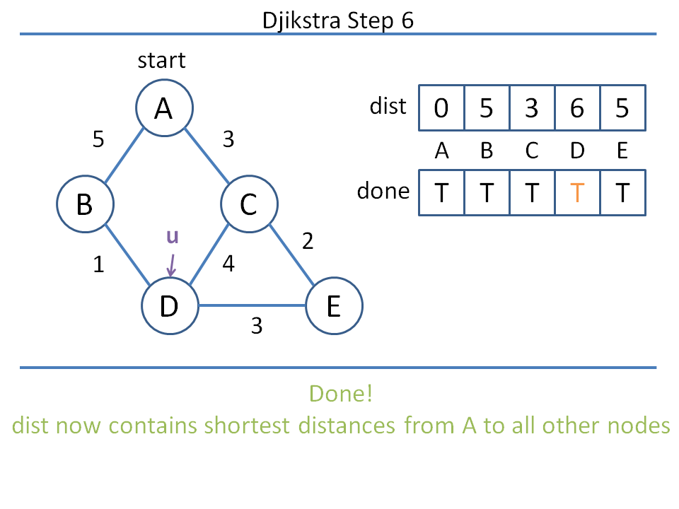
There are many variants of Djikstra's algorithm, some suited for different purposes than a general shortest-distance computer, but the gist is the same of each: a procedural way of finding shortest distances between nodes in a graph.
And that's Djiksta's algorithm!
Massive Review
How about a nice massive review to wind us down?
For each of the following sorts and data structures, provide a description and time complexity (if appropriate) for the operations and case analyses:
Sorts
Bubble Sort
Best Case |
Avg. Case |
Worst Case |
Stable? |
|---|---|---|---|
|
Click for answer.
|
Click for answer.
|
Click for answer.
|
Click for answer.
|
Insertion Sort
Best Case |
Avg. Case |
Worst Case |
Stable? |
|---|---|---|---|
|
Click for answer.
|
Click for answer.
|
Click for answer.
|
Click for answer.
|
Merge Sort
Best Case |
Avg. Case |
Worst Case |
Stable? |
|---|---|---|---|
|
Click for answer.
|
Click for answer.
|
Click for answer.
|
Click for answer.
|
Quick Sort
Best Case |
Avg. Case |
Worst Case |
Stable? |
|---|---|---|---|
|
Click for answer.
|
Click for answer.
|
Click for answer.
|
Click for answer.
|
Heap Sort
Best Case |
Avg. Case |
Worst Case |
Stable? |
|---|---|---|---|
|
Click for answer.
|
Click for answer.
|
Click for answer.
|
Click for answer.
|
Data Structures
Dynamic Arrays (STL vector)
Good for: |
Bad for: |
|---|---|
|
Click for answer.
|
Click for answer.
|
Linked Lists (STL list)
Good for: |
Bad for: |
|---|---|
|
Click for answer.
|
Click for answer.
|
Stacks (STL stack)
Good for: |
Bad for: |
|---|---|
|
Click for answer.
|
Click for answer.
|
Queues (STL queue)
Good for: |
Bad for: |
|---|---|
|
Click for answer.
|
Click for answer.
|
Binary Search Trees (STL set, map)
Good for: |
Bad for: |
|---|---|
|
Click for answer.
|
Click for answer.
|
Hash Tables (STL unordered_set)
Good for: |
Bad for: |
|---|---|
|
Click for answer.
|
Click for answer.
|
Heaps
Good for: |
Bad for: |
|---|---|
|
Click for answer.
|
Click for answer.
|
Having the Right Stuff
The whole point about learning all of these different data structures and algorithms is so that we can choose the right candidate for the right job.
As we've seen, some data structures and algorithms are better suited for some scenarios than others... let's examine a couple of those scenarios below.
Solutions to most of the below can be found here, in this week's classwork section.
Data Structures
Scenario 1: In the year 3000 (following the fall of mankind to the great Forney Industries Fembot Malfunction), you (who have somehow survived until then) are tasked with developing tracking chips to implant in the loyal subjects of your dystopian hegemony (OK, so I might be writing a book on this). These tracking chips have very little storage, and must be able to able to look for and possibly add a new contact for an individual in (at most) log(n) time.
Can you suggest a data structure to be used for this purpose? Fun fact, the c++ STL collections made it to the year 3000, which of them might you employ?
Scenario 2: Before the collapse of society, Forney Industries developed TriageBot 4000, a robot designed to assess the severity of hospital patients' maladies and begin treatment on those with the worst. It maintained a collection of waiting patients and was required to instantaneously determine who was most in need of the next available doctor.
What data structure would best accomplish TriageBot 4000's collection of patients?
Scenario 3: One of the more popular inventions of Forney Industries was a geneticist family-tracking robot called the GENEy. It was employed by the Census bureau to make sure that your reported family members were indeed related to you. Its job: canvas neighborhoods and organize People (capitalized to indicate it as a class) by their family name. It was required to track last names of families and organize each family member sequentially (though not in any particular order within the family).
What data structure would best track each family by their last name and organize each family's constituent People sequentially? Quick (at most O(log(n))) lookup and insertion of family members required.
Scenario 4: You are in charge of managing a prison for the political dissidents of the Forney Industries Empire. Prisoners are kept in isolation so as not to develop escape plans or further slander the great Forney Industries name. The one time that Prisoners are not in isolation is during meal times, during which you want to track who speaks with whom, and how often. You must design a system that can instantaneously find or place a Prisoner in one of your solitary-cells, and furthermore, in at most log(n) time determine how many times a Prisoner has spoken to another at mealtime. As a side-note, your prison is always at max-capacity.
Firstly, what container best stores the Prisoners in their cells? Secondly, what data structure internal to a Prisoner will best store their contacts? You need not worry about sorting either the Prisoners nor their contacts, but your data structures should *waste no space.*
Scenario 5: One of the more mundane inventions that came from Forney Industries was the SparkleMaster 2k, an industrial dish-washing robot designed to take large groups of dishes, clean them, and then file them into their proper kitchen locations. It received dishes in stacks on a conveyer-belt, and would need to clean each dish in a stack before moving to the next. After cleaning a dish, it would assess the dish's size, shape, and color, and have the instantaneous knowledge of which cabinet to place it in. Within a cabinet, dishes must be sorted from largest (on the bottom) to smallest (on the top).
What data structure should you use to model the sequence of washing from the inbound conveyer-belt? What data structure should you use to model the plate storage? You may need to use compound data-structures for each task.
Design Triage
Scenario 1: You are in charge of the M.E.R.I.C.A-S.T.A.R-S.P.A.N.G.L.E missile defense system (no one knows what the acronym stands for) that must assess which, out of some collection of missiles, is the closest, and target that first. Your simulations suggest that as long as you're able to sort the missile distances for destruction in n*log(n) time or less, the nation will be safe.
Which sort that we've learned about would you *not* want to pick for this task? Why?
Scenario 2: You have been tasked with creating a new map app... a mapp... called Cartographer using the abstract data type of a graph with locations separated by distances. With your new graph knowledge, you decide to represent your graph as an adjacency matrix with distances connecting two elements. Cartographer maps landmarks around the globe that are connected by roads.
What is wrong with your design approach, and what can you instead use to be more efficient?
Scenario 3: You decided to get clever and reduce collisions in your hash table by making your buckets hash tables themselves (the second level of which has buckets that are lists)! Triumphantly, you sit back in your chair for being so damn smart, but then run your code and discover that you have the same number of collisions that you had before!
What did you forget to do that made this approach problematic?
Scenario 4: You are a programmer prone to frequent bouts of selective amnesia. Unfortunately, today you've forgotten how to use recursion... entirely. Just your luck, your boss comes in and asks you to complete a task requiring a breadth-first traversal of some trees.
What technique or data structure could you use to perform the breadth-first traversal using iteration instead of recursion?
Scenario 5: Inspired by the last project, you've decided to reinvent the spell checker in a very compact manner. You've shrewdly determined that it's possible to represent words in a tree with insertion and lookup that is linear *for the size of the word,* which, if you're considering standard English, could be held beneath a constant that is the size of the longest English word.
Describe how you would structure the tree, and how you would use it to perform insertion and lookup that is linear in the size of the query word. In what ways is this technique superior to the hashtable implementation?
General Practice
Generate the heap that would be formed with the insertion ordering: 5, 22, 19, 10, 10, 10, 3, 2. Express your final answer in array form.
Insert nodes into a binary search tree in the order: 5, 10, 0, 15, 20. Pretending this is now an unbalanced AVL tree, where would a rotation
occur and what would the new, balanced AVL tree look like?
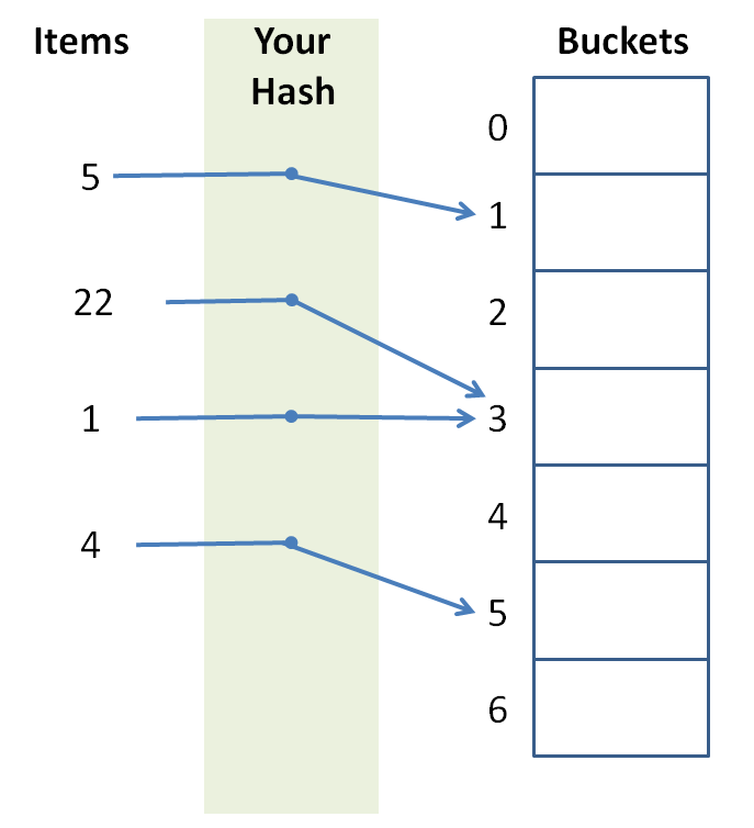
Design a hash function that elicits the following behavior:
Coding Practice
These examples, and other good ones if you're interested, were taken from CareerCup.com.
You are given a square grid of characters (we'll call it a maze), and a query string to find by an omni-directional path traversal in the maze. Your task is to count the number of times that you could form the query string by starting anywhere in the maze and moving in any of the four cardinal directions: N, E, S, and W. For example:
  const int GRID_SIZE = 4;

  int main () {
      char maze[GRID_SIZE][GRID_SIZE] = {
          { 'S', 'N', 'A', 'S' },
          { 'B', 'A', 'K', 'E' },
          { 'B', 'K', 'A', 'N' },
          { 'S', 'E', 'B', 'S' }
      };

      // Prints 5
      cout << countOccurences(maze, "SNAKES") << endl;
  }
To solve this, you'll complete the function signatures provided below, one of which counts all of the occurences in the grid, and the other that counts all of the occurences starting at a given row and column:
  // Counts all occurences in the grid starting at row r
  // and column c
  int occurences (char maze[][GRID_SIZE], string query, int r, int c) {
      // ... YOUR CODE HERE ...
  }

  // Counts all occurences in the grid
  int countOccurences (char maze[][GRID_SIZE], string query) {
      // ... YOUR CODE HERE ...
  }
You are given two sorted arrays of N > 0 positive, unique (i.e., no repeats amongst either array) integers. Provide a function median, as
given by the skeleton below, that computes the median value of a hypothetical third, sorted array composed of the elements of the 2 input arrays combined in O(log(n)) time.
  // Example usage
  int main () {
      {   // Prints 1.5
          int a[] = {1};
          int b[] = {2};
          cout << median(a, a+1, b, b+1) << endl;
      }
      {   // Prints 2.5
          int a[] = {2, 4};
          int b[] = {1, 3};
          cout << median(a, a+2, b, b+2) << endl;
      }
      {   // Prints 3.5
          int a[] = {1, 3, 5};
          int b[] = {2, 4, 6};
          cout << median(a, a+3, b, b+3) << endl;
      }
  }
  // Function signature:
  // b1 = beginning of array 1, e1 = end of array 1
  // same for b2, e2 for second array
  double median (int* b1, int* e1, int* b2, int* e2) {
      // ... YOUR CODE HERE ...
  }
Final
Closed notes! Closed everything!
I suggest you consider the following computational complexity cheat sheet!
You're going to do fine, breathe deep, focus on your problems, and try not to look at the giant, ticking, countdown clock unless absolutely necessary.
Goodbye but not Farewell
A special thank you for everyone who attended discussions -- you've been a pleasure to teach. It was an honor and a privilege to get to know you all.
Don't be a stranger; you'll probably see me in the office hours room for awhile to come!
Now... have you filled out your TA evals yet? :)