AI Probability Overview
So you want to do some cool stuffs in AI huh? Well for that... you're gonna need some maths...
Here's what this guide gets you:
An *at a glance* description of the results from the lectures in AI
Important formulas alongside their purposes
A good review guide for exams
Warning: the content here is not meant in-place of the more thorough explanations from the lectures! It's important to understand the context of each result that follows.
Motivation for Probs and Stats in AI
So how'd we get here? Why suddenly do we need probs and stats for automated agents?
Well, consider how we did things in the strictly logic- / knowledge-based agents.
KB:
"If it is raining, then the sidewalk will be wet"
1. \(R \Rightarrow S \equiv \lnot R \lor S\)
"The sidewalk is dry"
2. \(\lnot S\)
Problem: Dealing with uncertainty
Although the above will be fine for making definitive conclusions about the sidewalk's wetness under these precise rules and facts, there are a number of issues it's ill-equipped to handle with formal logic alone.
What if the KB is missing parts of the rules? e.g., that if it's raining AND the sidewalk is uncovered, THEN it will be wet?
What if we lack observations to use those rules? If the premises of an implication are unsatisfied, we can't make any statements about the conclusion.
What if we want to add-to or change the rules later? We would have to individually sift through all of the relevant sentences and make those changes.
KB construction is entirely top-down: we, the programmer, construct the sentences, and cannot (in general) automagically harvest them from data / nature.
Idea: perhaps we can rethink how we represent "the way the world works" as a bunch of boolean sentences, since those are hard to scale and deal with uncertainty.
Distributions
Instead of truth tables / logical sentences to establish which worlds are still possible given what we know, we can instead think about how likely / probable a given world or set of variables are given what we know.
A probability distribution maps some set of worlds to their probability of being observed.
Joint probability distributions tables, specified via \(P(A \land B \land C \land ...) = P(A, B, C, ...)\) define the likelihood of seeing event \(A \land B \land C \land ...\) for all variables and their associated values.
Observe the following joint distribution over our Solicitorbot example's variables: L (whether or not a house's lights are on) and H (whether anyone is home).
World |
L |
H |
\(P(L, H) = P(L \land H)\) |
|---|---|---|---|
\(w_0\) |
0 |
0 |
\(P(L = 0, H = 0) = 0.30\) |
\(w_1\) |
0 |
1 |
\(P(L = 0, H = 1) = 0.10\) |
\(w_2\) |
1 |
0 |
\(P(L = 1, H = 0) = 0.10\) |
\(w_3\) |
1 |
1 |
\(P(L = 1, H = 1) = 0.50\) |
Think of joint distributions as the way of modeling how often each variables' values co-occur WITHOUT making any observations / before gathering any evidence.
Vocabulary & Notation
Think of the notation \(P(A, B, C)\) as a function called
Pthat, for parameters being variables, returns some probability of seeing that combination of variable values.If all of those arguments are assigned a value, we're targeting a particular row in that distribution, e.g., \(P(L = 1, H = 0) = 0.10\) refers to the row of world \(w_2\) in the Solicitorbot joint above.
If any of those arguments are left unassigned, it means the result will not be a single probability value, but rather, a table consisting of all values of the unassigned variable. E.g., \(P(H, L=0)\) would refer to a table consisting of rows / worlds \(w_0, w_1\) because those are the ones with \(L=0\) and we would return all values of the unassigned variable \(H\), viz., \(P(H=1, L=0), P(H=0, L=0)\)
A joint distribution \(P(A, B, C)\) is called the full joint if the arguments to
Pare the set of ALL variables in the system. E.g., \(P(L, H)\) is the full joint of the example above because the only variables in the system are \(\{L, H\}\)A joint distribution is called a joint marginal if it includes 2 or more variables that are NOT the full set of variables in the system.
Axioms of Probability
Probability Value Range: All probability values assigned to any given world \(w\) must range between 0 (impossible) and 1 (certain), inclusively: $$0 \le P(w) \le 1$$
The sum of all probability values in worlds \(w\) that are possible must sum to 1: $$\sum_w P(w) = 1$$
Law of Total Probability: The probability of any subset of variables, \(\alpha\), is the sum of every possible world \(w\) that in that subset's models: $$P(\alpha) = \sum_{w \in M(\alpha)} P(w)$$
We can quickly verify that the first two axioms are met by our Solicitorbot joint probability table above, but consider the following:
What is the raw probability (i.e., the prior) that someone is home? In other words, what is \(P(H = true)\)?
Using the third axiom above, we see that: $$P(H = 1) = \sum_{w \in M(H = 1)} = P(w_1) + P(w_3) = 0.60$$
A direct consequence of the Law of Total Probability is known as marginalization whereby a variable \(B\) can be "marginalized" / removed from a joint distribution by summing over its values OR introduced into a joint (depending on whether we're moving from the right-hand-side to the left or vice versa in the equation below): $$P(A) = \sum_b P(A, B=b)$$
Suppose we want to get the distribution \(P(H)\) from the joint \(P(H, L)\), thereby "marginalizing" \(L\) (and remembering that we already found \(P(H=1)\) above).
\begin{eqnarray} P(H = 0) &=& \sum_l P(H = 0, L = l) \\ &=& P(H=0, L=0) + P(H=0, L=1) \\ &=& 0.3 + 0.1 \\ &=& 0.4 \end{eqnarray}
Conditional Distributions
Joint distributions tell us the relationships between variables prior to observing anything about the world, which is still useful if we never take in any observations... but what if we do?
A conditional probability distribution specifies the probability of some query variables \(Q\) given observed evidence \(E=e\), is expressed: $$P(Q | E=e) = P(Q | e)$$
Some notes on that... notation:
The bar | separating \(Q\) and \(E=e\) in \(P(Q | E=e)\) is known as the "conditioning bar" and is read as "given", e.g., "The likelihood of Q given E=e"
The query variables are what still have some likelihood attached to them, but now under the known context of the evidence (assumed to be witnessed with certainty, which is why they're assigned \(E=e\))
Formally, Observations / Evidence constrain the set of possible worlds in probabilistic reasoning by assigning a probability of 0 to worlds that are inconsistent with the evidence.
Suppose, in the Solicitorbot example, that the lights are observed to be off, i.e., \(P(L = false = 0)\). This would have the following effect on our joint:
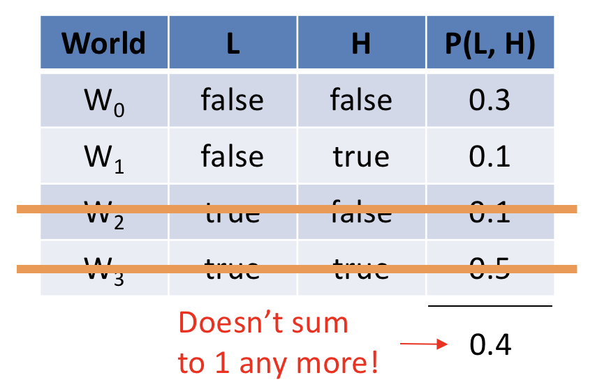
To re-normalize the remaining, still-possible rows, we simply divide by the probability of the evidence that was observed to construct a conditional distribution.
Conditioning: for any two sets of queries and evidence we thus have: $$P(Q | e) = \frac{P(Q, e)}{P(e)} = \frac{\text{joint prob of \{Q, e\}}}{\text{prob. of \{e\}}}$$
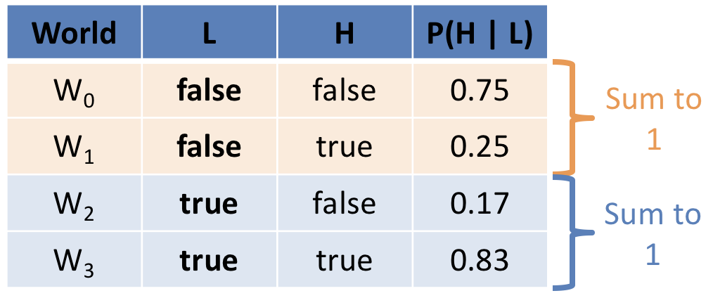
Noting that the probability of our evidence \(P(L = 0) = 0.4, P(L = 1) = 0.6\), we can apply conditioning to each of our joint rows \(P(L, H)\), which allows us to create the conditional distribution \(P(H | L)\):
Notes on the above:
The purpose of this distribution now tells us the likelihood that someone's home ONCE WE OBSERVE the state of the house's lights (i.e., updated for that evidence).
Notice that the rows here are different than in the joint; in general: \(P(L, H) \ne P(H | L)\) for any variables.
In the joint distribution, the sum of ALL rows was always 1, but in the conditional, note that the summing-to-one axiom is preserved WITHIN each condition of the evidence.
Recap: if we have the full joint distribution, the conditioning operation gives us a formula for finding the likelihood of ANY query given ANY evidence that's been observed, allowing our agent to dynamically assess the likelihood of certain worlds or events.
Independence
Problem: Conditioning requires the joint distribution over variables to answer any arbitrary conditional query of the format \(P(Q|e)\), and the full joint is too large to store in memory for even modestly-sized systems.
Idea: Find a way to break the joint into smaller factors, which could then be used to reconstruct only the parts of the joint that are needed to answer queries.
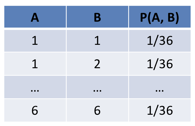
Inspiration: Suppose we roll two, fair, 6-sided die: \(A, B\). Will the outcome of \(A\) tell me anything about the outcome of \(B\)? In other words, does treating \(A\) as evidence update my beliefs about \(B\)?
No, A and B are irrelevant to one another, which allows us to break the joint apart into smaller pieces.
Some notes:
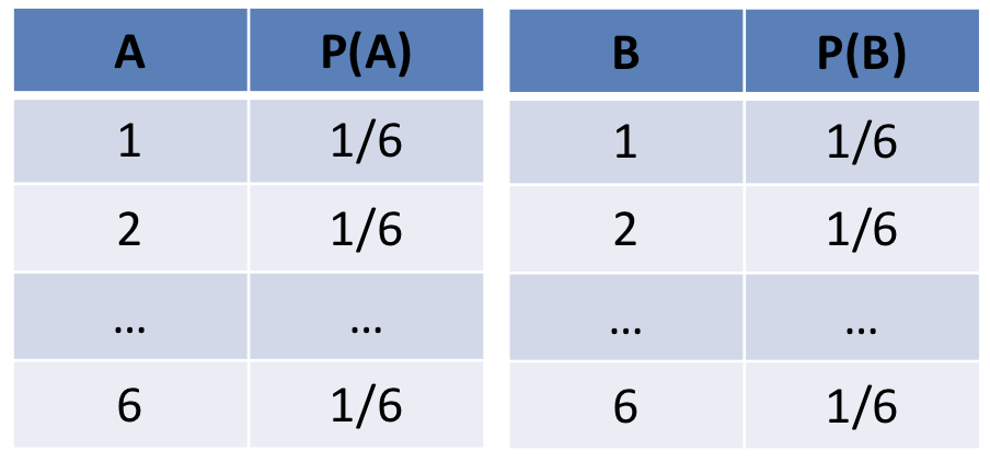
Above, \(P(A|B) = P(A)\) and \(P(B|A) = P(B)\) because A and B tell us nothing about one another -- they're independent dice rolls.
The original joint had 36 rows, and each individual table \(P(A)\), \(P(B)\) have 6 rows each (12 total, less than 36). Since A and B are independent, we can instead represent the joint as a product of each individual variable's distribution to save room.
Two variables \(A, B\) are said to be independent, written \(A \indep B\), if and only if the following holds: $$A \indep B \Leftrightarrow P(A | B) = P(A) \Leftrightarrow P(B | A) = P(B)$$
Joint Independence Factoring: a consequence of independence: for two variables \(A, B\): $$A \indep B \Leftrightarrow P(A, B) = P(A) P(B)$$
Recap: if we can find independence relationships between variables in our system, we can break the joint distribution down into smaller pieces (not needing to store the entire, massive full joint) and can reconstruct any rows we want by simply multiplying together the factors.
Problem: Two variables that were once independent can be made dependent when given a third variable / set of variables, or vice versa.
So called conditional dependence / independence presents a problem for breaking the joint up into smaller pieces.
Suppose we have a third variable \(S\), representing the sum of the individual dice rolls, i.e., \(S = A + B\)
We know that \(A \indep B\), but suppose I told you the outcome of \(A = 6\) and the sum of the dice rolls \(S = 7\). Does knowing about \(S, A\) change our belief about \(B\)?
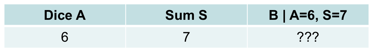
Yes! If I told you that \(A = 6\) and \(S = 7\), then you should infer that \(B = 1\).
Curiously, above we have a scenario wherein \((A \indep B)\) but \((A \not \indep B | S)\).
Bayesian Networks
Problem: in large systems of variables, modeling which variables are independent given what other variables is tricky and requires that we have a way of encoding 1) the independence / conditional independence relationships in the system and then 2) the probabilities associated with each variable necessary to reconstruct the full joint.
A Bayesian Network is a data structure used in probabilistic reasoning to encode independence relationships between variables in the reasoning system, and is composed of:
Structure: a Directed Acyclic Graph (DAG) in which nodes are Variables and edges (intuitively) point from causes (parents) to their direct effects (children): $$[Cause] \rightarrow [Effect]$$
[!] While the above directionality helps us to think about the structure, sometimes the relationship is non-causal in Bayesian Networks, and an edge \(X \rightarrow Y\) simply means that \(X \not \indep Y\)
Probabilistic Semantics: conditional probability distributions (or tables, in the case of discrete variables, known as CPTs) associated with each node of the format: $$P(V | parents(V)) ~ \forall~V$$ ...which is intuitively structured as: $$P(effect~|~causes)$$
It is assumed that the network structure is a faithful representation of the independence relationships that would be represented in reality / some collected dataset underpinning the probability values that would be found in the full joint.
If so, we have a recipe for breaking the full joint down into its constituent pieces.
The Markovian Factorization of the FULL joint distribution \(P(V_1, V_2, V_3, ...)\) in some Bayesian Network is: \begin{eqnarray} P(V_1, V_2, V_3, ...) &=& \prod_{V_i \in \textbf{V}} P(V_i~|~parents(V_i)) \\ &=& \{\text{Product of all CPTs in the BN}\} \end{eqnarray}
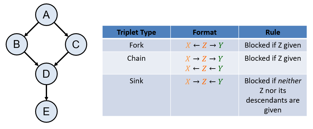
Directional Separation (d-sep)
The rules of directional-separation (d-separation = d-sep) determine a Bayesian Network's independence and conditional independence claims directly from the network's structure.
  # Returns true if X is independent of Y given Z, else false
  d_sep(X, Y, {Z}):
      for each undirected path p between X and Y:
          openPath = true
          for each triplet t along p:
              if t is blocked:
                  openPath = false
                  break
          if openPath:
              return false
      return true
Bayesian Network Inference
Probabilistic inference is the process of finding a query of the format \(P(Q|e)\) using the structure and semantics of a Bayesian Network.
Some queries of this format can be answered easily if the query is (1) one of the CPTs in the network, (2) can be reduced, via d-sep, to one such CPT, or (3) is simply a row of the joint... for everything else, there's:
Enumeration Inference is an inference algorithm that can compute any query via sums-of-products of conditional probabilities from the network's CPTs.
The roadmap by which it does this for Query variables \(Q\), evidence \(E = e\), and hidden variables \(Y\) (anything not \(Q, e\)):
$$\begin{eqnarray} P(Q~|~e) &=& \frac{P(Q, e)}{P(e)}~ \text{(Conditioning)} \\ &=& \frac{1}{P(e)} * P(Q, e)~ \text{(Algebra)} \\ &=& \frac{1}{P(e)} * \sum_{y \in Y} P(Q, e, y)~ \text{(Law of Total Prob.)} \\ \end{eqnarray}$$ Observe that \(P(Q, e, y)\) is the full joint distribution, which we know how to factor into the CPTs using the Markovian Factorization!
To efficiently / formulaically solve any query, we can perform enumeration inference by hand through the following steps:
Step 1: Identify Variable Types: label the variables in the network as one of the three categories: Query variables \(Q\), evidence \(E = e\), and hidden variables \(Y\) (anything not \(Q, e\))
Step 2: Compute \(P(Q, e) = \sum_{y \in Y} P(Q, e, y)\). Solving for the joint \(P(Q,e)\) allows us to easily solve for the probability of the evidence (step 3) and then normalize by it in the final step.
Step 3: Find \(P(e) = \sum_{q \in Q} P(Q, e)\). In other words, find \(P(e)\) by summing over all of the values you found in step 2.
Step 4: Normalize \(P(Q | e) = \frac{P(Q, e)}{P(e)}\). In other words, divide step 2 by step 3 to find the answer to your query. Voila!
Recap: Bayesian Networks are compact / parsimonious representations of the full joint distribution that intuitively structure the relationships between variables in terms of cause-effect relationships, and with algorithms that can be used to answer any query without needing the full, often massive, joint.
Utility
Problem: although Bayesian Networks / Probability Theory give us ways to extend / generalize the inference capabilities of knowledge-based systems, we still need a way by which an intelligent agent could use such a system to make autonomous decisions.
Idea: borrow the notion of utility theory from philosophers like Mills / algorithms like Minimax for game playing.
A Utility Function, \(U(s, a) = u\), maps some state \(s\) and action \(a\) to some numerical score \(u\) encoding its desirability (a higher \(u\) is more desirable -- and no, that's not some sort of ad for drugs).
Problem: the states our utility function will score / evaluate are not always equally likely (think: lotter tickets).
Idea: weight those utility scores by the likelihood of seeing them.
The Expected Utility (EU) of some action \(a\) given any evidence \(e\) is the average utility value of the possible outcome states \(s \in S\) weighted by the probability that each outcome occurs, or formally: $$EU(a | e) = \sum_{s \in S} P(s | a, e) * U(s, a)$$
The Maximum Expected Utility (MEU) criterion stipulates that an agent faced with \(a \in A\) actions with uncertain outcomes (and any observed evidence \(e\) shall choose the action \(a^*\) that maximizes the Expected Utility, or formally: $$MEU(e) = max_{a \in A} EU(a | e)$$ $$a^* = \argmax_{a \in A} EU(a | e)$$
Decision Networks
Problem: as an agent's system of knowledge / interconnected variables and decision points grows complex, it's difficult to proceduralize EU / MEU computations without some structure of what influences what.
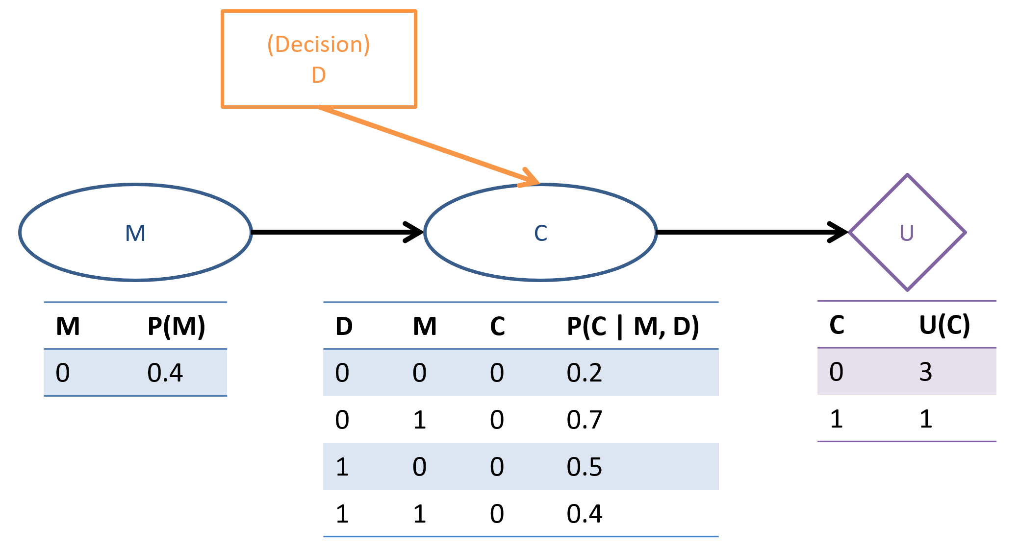
A decision network unifies the stochastic modelling capacities of a Bayesian network with action-choice and utility theory by adding two additional nodes to the Bayesian network model. In particular, decision networks specify:
Chance Nodes (Circles) are traditional Bayesian Network variable nodes encoding chance in CPTs.
Decision Nodes (Rectangles) represent choices that the agent has to make, and can be used to model influences on the system. In certain contexts, decision nodes are referred to as interventions.
Decision nodes behave as follows:
Decisions have no CPTs attached to them; all queries to a decision network are assumed to have each decision node as a "given" since we are considering the utilities of different decisions.
Though treated like evidence in other CPTs, we do not need to normalize by their likelihood.
Utility Nodes (Diamonds) encode utility functions, wherein parents \(pa\) of utility nodes are the arguments to the utility function, \(U(pa)\).
Decision networks provide a more general formula for evaluating EU queries, translating the original formula if we designate \(pa(U)\) to be the chance node parents of the utility node in the network:
\begin{eqnarray} EU(a | e) &=& \sum_{s \in S} P(s | a, e) * U(s, a) \\ &=& \sum_{p \in pa(U)} P(p | a, e) * U(p, a) \end{eqnarray}
Computing EU within a DN
The process for computing the EU using a DN is as follows:
Step 1: Compute \(P(S | A, e)\). Notably, leaving \(S, A\) capital here means we compute this FOR ALL values of our chance node parents of the utility node (\(S\) in the original EU equation) and all possible actions \(a \in A\) our agent has.
Note: this is where we would use the Bayesian Network / chance nodes to compute the value of this query, or by-hand if, say, on an exam (poor souls).
Step 2 - Find \(EU(A | e) = \sum_s P(s | a, e) U(s, a)~\forall~a\). The \(P(s | a, e)\) expressions will come from step 1 and the \(U(s, a)\) values from the decision network, directly.
Step 3 - Find \(MEU(e) = max_{a \in A} EU(a | e)\) and \(a^* = \argmax_{a \in A} EU(a | e)\). Just pick the largest value you found in step 2, and the action that generated it is your agent's choice!
Value of Perfect Information
Problem: sometimes, evidence / observations that might help our agent make a good decision are unknown to it and obtaining that information may come at a cost. We need a means of quantifying curiosity to determine if the "juice is worth the squeeze" in obtaining that info.
Computing the Value of Perfect Information (VPI) of observing some variable \(E'\) for any *already* observed evidence \(E = e\) is defined as the difference in maximum expected utility between knowing and not knowing the state of \(E'\), written: $$VPI(E' | E = e) = MEU(E = e, E') - MEU(E = e)$$
In words, interpreting the above:
\(VPI(E' | E = e)\) = The value of learning about the state of \(E'\) if I already know \(E = e\).
\(MEU(E = e, E')\) = The maximum expected utility of me acting optimally knowing what I do now \(E=e\), AND about the state of \(E'\).
\(MEU(E = e)\) = The maximum expected utility of me acting optimally knowing what I do now \(E=e\) (WITHOUT the variable I'm evaluating, \(E'\)).
This computation would be relatively straightforward (just a couple of MEU computations like we did above) were it not for a couple of snags:
We have to assess how each value of the evaluated variable \(E'\) affects our decisions and the resulting utility (we might change our mind given some new evidence).
Since \(E'\) is still a random variable, we need to weight our final assessment according to the likelihood of seeing each value of \(E'=e'\) given our already observed evidence \(E = e\).
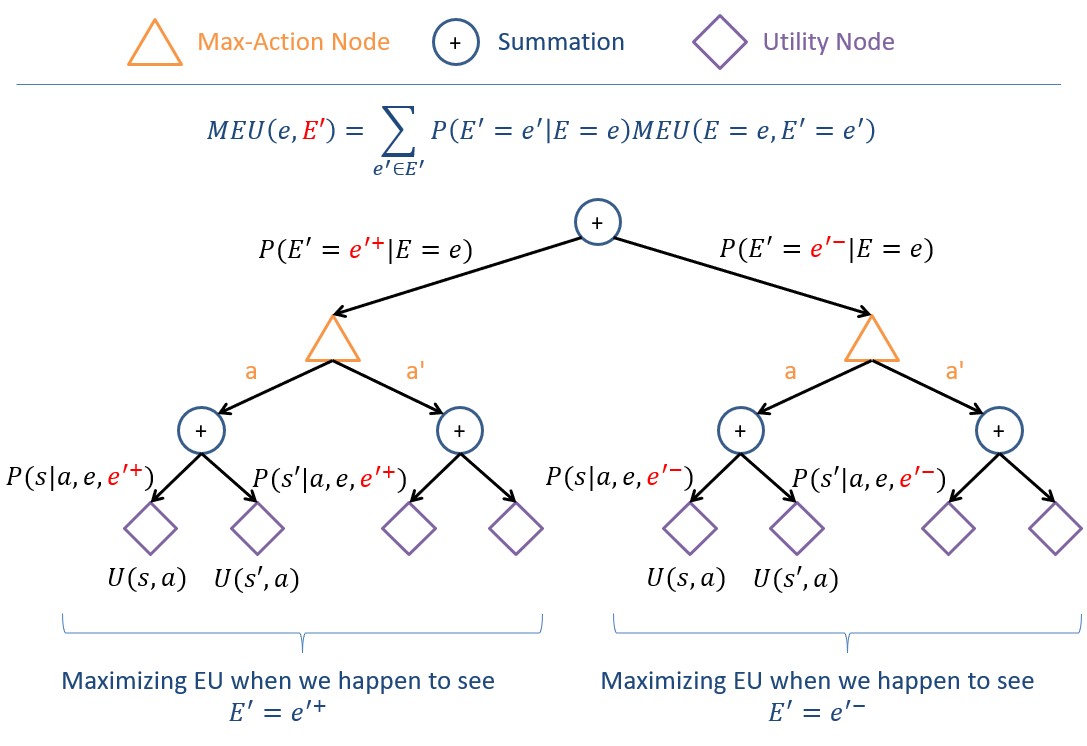
The Maximum Expected Utility associated with the reveal of some variable \(E'\) given some other evidence \(E = e\) is the weighted sum over all values \(e' \in E'\) of the likelihood of seeing \(e'\) with the MEU of how we would act seeing \(e'\), or formally: $$MEU(E = e, E') = \sum_{e' \in E'} P(E' = e' | E = e) MEU(E = e, E' = e')$$
Visualized in an image I see past-me named meu-madness.png.
Proceduralized, we can compute the \(VPI(E' | E=e)\) on any given decision network through the following steps:
Step 1 - Find \(P(S | A, e)\) AND \(P(S | A, e, e')\). Note again, this is for all state \(S\) and action \(A\) values since those are left capital.
Step 2 - Find \(EU(A|e)\) AND \(EU(A|e, e')\). These will come from Step 1's probabilistic queries and the utility function's scores.
Step 3 - Find \(MEU(E=e)\) AND \(MEU(E=e, E')\). These will come from Step 2. Remember to use the "unknown variable" form of MEU above for the \(MEU(E=e, E')\) term.
Step 4 - Find \(VPI(E' | E=e) = MEU(E = e, E') - MEU(E = e)\). Plug and chug from Step 3!
Formulas
Is the above even too long for you to read? Fine, here's the meat.
Name |
Formula |
Purpose |
|---|---|---|
Law of Total Probability (LoTP) |
The probability of any subset of variables, \(\alpha\), is the sum of every possible world \(w\) that in that subset's models: $$P(\alpha) = \sum_{w \in M(\alpha)} P(w)$$ |
Finding the likelihood of some conjunctive sentence \(\alpha\) over its consistent worlds. |
Law of Total Probability (LoTP) - Marginalization |
Alternate way of thinking about LoTP such that a variable \(B\) can be "marginalized" / removed from a joint distribution by summing over its values OR introduced into a joint (depending on whether we're moving from the right-hand-side to the left or vice versa in the equation below): $$P(A) = \sum_b P(A, B=b)$$ |
Adding or removing variables from a joint probability expression. |
Conditioning |
For any query variable \(Q\) and evidence \(E = e\): $$P(Q | e) = \frac{P(Q, e)}{P(e)}$$ OR (going the opposite direction) $$P(Q, e) = P(Q|e)P(e)$$ |
Converting between joint and conditional distributions by accounting for the probability of the evidence. |
Independence |
Two variables \(A, B\) are said to be independent, written \(A \indep B\), if and only if the following holds: \begin{eqnarray} A &\indep& B \Leftrightarrow P(A | B) = P(A) \Leftrightarrow P(B | A) = P(B)~\forall~a \in A, b \in B \\ A &\indep& B \Leftrightarrow P(A, B) = P(A) P(B) \end{eqnarray} |
Useful for simplifying conditional distributions by removing evidence that is irrelevant to the query (first equation), or by factoring joint distributions into smaller pieces (second equation). |
Conditional Independence |
Two variables \(A, B\) are said to be conditionally independent given some third set of variables \(C\) (written \(A \indep B~|~C\)) if and only if the following holds: $$A \indep B~|~C \Leftrightarrow P(A~|~B, C) = P(A~|~C)$$ |
Same idea as Independence above, but generalized for any known / observed evidence \(C\). Notice how this is exactly the same result as the first equation in independence except everything has a \(|C\) tacked on. |
Markovian Factorization |
The Markovian Factorization of the FULL joint distribution \(P(V_1, V_2, V_3, ...)\) in some Bayesian Network is: \begin{eqnarray} P(V_1, V_2, V_3, ...) &=& \prod_{V_i \in \textbf{V}} P(V_i~|~parents(V_i)) \\ &=& \{\text{Product of all CPTs in the BN}\} \end{eqnarray} |
Means of reconstructing any row of a Bayesian Network's joint distribution as a product of its individual CPTs / factors. Used in enumeration inference to turn any query into a function of the network's "known" probabilities: the CPTs. |
Expected Utility (EU) |
The Expected Utility (EU) of some action \(a\) given any evidence \(e\) is the average utility value of the possible outcome states \(s \in S\) weighted by the probability that each outcome occurs, or formally: $$EU(a | e) = \sum_{s \in S} P(s | a, e) * U(s, a)$$ |
Marries probability theory with utility theory to give agents a means of predicting the average desirability of an action. In a decision network, \(S\) represents the chance node parents of a utility node. |
Maximum Expected Utility (MEU) - All Known Evidence |
The Maximum Expected Utility (MEU) criterion stipulates that an agent faced with \(a \in A\) actions with uncertain outcomes (and any observed evidence \(e\)) shall choose the action \(a^*\) that maximizes the Expected Utility, or formally: $$MEU(e) = max_{a \in A} EU(a | e)$$ $$a^* = \argmax_{a \in A} EU(a | e)$$ |
Dictates that an agent's "best" decision \(a^*\) (no relation to the search algorithm) in given any evidential circumstance \(E=e\) should be the one that has the highest average utility. |
Maximum Expected Utility (MEU) - Unknown Variable \(E'\) |
The Maximum Expected Utility associated with the reveal of some currently unknown variable \(E'\) given some other known evidence \(E = e\) is the weighted sum over all values \(e' \in E'\) of the likelihood of seeing \(e'\) with the MEU of how we would act seeing \(e'\), or formally: $$MEU(E = e, E') = \sum_{e' \in E'} P(E' = e' | E = e) MEU(E = e, E' = e')$$ |
Used during computation of VPI to assess the weighted MEU average of a currently-unknown-valued variable \(E'\). |
Value of Perfect Information (VPI) |
Computing the Value of Perfect Information (VPI) of observing some variable \(E'\) for any *already* observed evidence \(E = e\) is defined as the difference in maximum expected utility between knowing and not knowing the state of \(E'\), written: $$VPI(E' | E = e) = MEU(E = e, E') - MEU(E = e)$$ |
Quantifies the rational price of curiosity -- how much utility (in expectation) some currently unknown variable \(E'\) is to our agent. |